MolMap

Visualizing Molecule Libraries as Topographic Maps

Martin Gronemann

, Michael J

unger

, Nils Kriege

and Petra Mutzel

Institut f

ur Informatik, Universit

at zu K

oln, K

oln, Germany

Dept. of Computer Science, Technische Universit

at Dortmund, Dortmund, Germany

Keywords:

Graph Drawing, Clustered Graphs, Topographic Maps, Drug Discovery, Molecule Libraries.

Abstract:

We present a new application for graph drawing and visualization in the context of drug discovery. Combining

the scaffold-based cluster hierarchy with molecular similarity graphs — both standard concepts in cheminfor-

matics — allows one to get new insights for analyzing large molecule libraries. The derived clustered graphs

represent different aspects of structural similarity. We suggest visualizing them as topographic maps. Since

the cluster hierarchy does not reﬂect the underlying graph structure as in (Gronemann and J

unger, 2012), we

suggest a new partitioning algorithm that takes the edges of the graph into account. Experiments show that the

new algorithm leads to signiﬁcant improvements in terms of the edge lengths in the obtained drawings.

1 INTRODUCTION

Drug discovery is a tedious and expensive process that

typically involves the experimental evaluation of large

compound libraries by high-throughput screening in

order to identify promising small molecules that bind

to a speciﬁc biological target. These compounds may

serve as a starting point for chemical modiﬁcations,

e.g., in order to reduce side effects or to improve

potency. A guiding principle during this process is

to elucidate and exploit the relationship between the

structure of a molecule and its biological properties.

In the course of the drug discovery process typi-

cally structural information on compounds as well as

experimental results are generated. Supporting the

drug discovery process based on this data by ade-

quate computational methods like, e.g., largely auto-

mated data mining algorithms, is a fundamental task

in cheminformatics (Brown, 2009). However, only

recently several sophisticated visual analysis tools for

this domain have been developed (Wetzel et al., 2009;

Klein et al., 2012; Lounkine et al., 2010; Strobelt

et al., 2012; Herhaus et al., 2009) with the aim to

allow the user to explore the chemical space and

make decisions based on his expert knowledge. These

tools often represent sets of molecules and their struc-

tural relations by means of graphs, and they rely on

graph drawing techniques for visualization. Since

structural relations are rather complex, different ap-

proaches have been developed, some of which orga-

nize molecules in a tree-like hierarchy while others

are based on pairwise similarities. The complexity of

structural relations, the amount of data and the differ-

ent perspectives chemists from different branches of

chemistry may have makes it difﬁcult to ﬁnd an ap-

proach that satisﬁes all needs.

Irwin recently summarized the problem as fol-

lows: “In principle, one would like to be able to or-

ganize and browse large chemical datasets [. . . ] as

easily as one can today browse maps on the inter-

net.” (Irwin, 2009) This comparison gives the im-

petus for our approach to represent molecule sets

by clustered graphs, which are then visualized as

topographic maps based on a method recently pro-

posed (Gronemann and J

unger, 2012). The use of

clustered graphs allows us to model different aspects

of structural similarity between compounds in a single

graph and to visualize them in one picture in which

similar molecules appear close to each other. Clus-

tered graphs have not yet been applied to visualize

chemical compounds, the most likely reason is that

drawing them is difﬁcult. This is caused by the re-

quirement to generate an appealing drawing of the

underlying graph that simultaneously represents the

hierarchy of nested subsets of its nodes. The issue

becomes especially challenging when the cluster hi-

erarchy does not reﬂect the “natural” clusters of the

underlying graph. This problem arises with our rep-

resentation of molecular data sets by clustered graphs

and was not addressed in (Gronemann and J

unger,

515

Gronemann M., Jünger M., Kriege N. and Mutzel P..

MolMap - Visualizing Molecule Libraries as Topographic Maps.

DOI: 10.5220/0004267205150524

In Proceedings of the International Conference on Computer Graphics Theory and Applications and International Conference on Information

Visualization Theory and Applications (IVAPP-2013), pages 515-524

ISBN: 978-989-8565-46-4

 2013 SCITEPRESS (Science and Technology Publications, Lda.)

2012). Therefore we develop a new partitioning pro-

cedure that exploits the degrees of freedom in the al-

gorithm with the goal to obtain shorter edges. In order

to meet the requirements of the application domain,

our procedure also supports the display of structural

formulae of compounds and the superimposition of

a heat map that allows the representation of property

values.

2 RELATED WORK

A straight-forward and wide-spread approach to

browse compound datasets are molecular spread-

sheets depicting compounds and their properties in

table form. Recently several more sophisticated tools

for the visualization of compound sets have been de-

veloped. Many of these represent chemical com-

pounds by means of graphs:

In (Wawer et al., 2008) the concept of ‘Network-

like Similarity Graphs’ was introduced to study

structure-activity relationships of small molecules.

Here, compounds are represented by nodes and two

nodes are connected by an edge if their compounds

exceed a certain similarity threshold. These graphs

are then visualized using a force-directed layout algo-

rithm (Fruchterman and Reingold, 1991). In addition,

similarities are used to derive a hierarchical cluster-

ing of all nodes. However, for visualization only a

single clustering is selected instead of displaying the

full hierarchy. The approach was implemented by the

open-source application SARANEA (Lounkine et al.,

2010) based on the framework JUNG

. A different

application, also based on pairwise molecular simi-

larities, is HiTSEE (Strobelt et al., 2012). This tool

maps compounds on the plane trying to preserve dis-

tances derived from similarities by Multidimensional

Scaling (MDS).

Several concepts to organize compounds via hi-

erarchical classiﬁcation schemes have been pro-

posed (Schuffenhauer and Varin, 2011). These are,

e.g., based on clustering algorithms or on domain spe-

ciﬁc methods based on rules incorporating chemical

knowledge. An approach of the second category is the

so-called scaffold tree (Schuffenhauer et al., 2007) on

which the visual analysis tool Scaffold Hunter (Wet-

zel et al., 2009; Klein et al., 2012) is based. For

visualization, a radial style tree drawing algorithm

is used. The tool MolWind (Herhaus et al., 2009)

is also based on the scaffold tree concept, but uses

NASA’s World Wind engine to map scaffolds to a vir-

tual globe. While MolWind is not directly related

http://jung.sourceforge.net

to graph drawing, we take up the MolWind idea to

map chemical information to intuitively understand-

able geographic representations, and realize it in the

realm of clustered graph drawing.

While clustered graph drawing is a lively research

topic in graph drawing (Sugiyama and Misue, 1991;

Huang and Eades, 1998) (see, e.g., in GDEA

), only

few approaches exist for drawing clustered graphs as

maps. Gansner et al. have suggested the use of ge-

ographic maps for enhancing clusters and visualiz-

ing similarities (Gansner et al., 2009; Gansner et al.,

2010). They ﬁrst compute a partition of the nodes by

applying a cluster algorithm, then use a force-directed

method or MDS to compute a layout, and ﬁnally use

both to create a colored map. The combination of

the layout and clustering methods used for generating

the map, plays an important role regarding the visual

shape of the clusters in the ﬁnal layout. In order to

obtain a map where the countries form compact ar-

eas, requires that the result produced by the layout

algorithm matches the partitioning of the clustering

step. Otherwise, the partitions are visually scattered,

this problem is referred to as fragmentation.

An alternative approach for visualizing hierarchi-

cally clustered graphs as topographic maps has been

suggested recently in (Gronemann and J

unger, 2012).

Topographic maps have a long history in information

visualization. Mostly used for visualizing point dis-

tributions, they offer a natural way to explore data.

In (Fabrikant et al., 2010) the effect of using to-

pographic maps as metaphor is studied. They conﬁrm

the usage of elevation levels as an effective way to en-

code similarities. Gronemann and J

unger propose to

represent the complete hierarchy of a clustered graph

by elevation levels. The elevation model is deﬁned

such that nodes in different subtrees are separated by

a valley. In other words, nodes in the same cluster

are placed together on a plateau. This simple idea

requires that the layout algorithm generates compact

areas for all clusters.

By using a treemap approach for the layout the

problem of fragmentation is avoided. Several meth-

ods for generating treemaps exist in the literature.

Starting with the work of (Johnson and Shneiderman,

1991), where a hierarchy is mapped on a space ﬁll-

ing curve, most algorithms are based on a rectan-

gular subdivision scheme. A good overview over

the vast amount of treemap techniques can be found

in (Schulz, 2011).

Graph Drawing E-Print Archive,

http://gdea.informatik.unikoeln.de/

IVAPP2013-InternationalConferenceonInformationVisualizationTheoryandApplications

516

3 COMPOUND LIBRARIES

AND CLUSTERED GRAPHS

A clustered graph is a tuple (G,T ), where G = (V,E)

is graph and T = (V

) is a rooted tree such that

the leaves of T are the nodes in V . Each inner node

v of T corresponds to a cluster of G comprising all

leaves of the subtree rooted at v. Therefore the inner

nodes of T are called cluster nodes, T is referred to as

cluster tree and deﬁnes a hierarchy of nested subsets

of V .

Approaches to explore chemical compound li-

braries typically allow the user to navigate between

regions of molecules with a similar structure. We

combine two orthogonal concepts from cheminfor-

matics to derive clustered graphs that represent two

different aspects of structural similarity.

3.1 Molecular Similarity Graph

A set of compounds with pairwise similarities can

be represented by a graph: Molecules are associated

with nodes and two nodes are connected by an edge

if their similarity exceeds a certain threshold. This

approach is applied in, e.g., (Wawer et al., 2008;

Lounkine et al., 2010). We additionally annotate

edges with the corresponding similarity values. For

a given set of molecules M we deﬁne a similarity

graph G(M) = (V,E) with edge weights w according

to V = M, E = {(u, v) ∈ V × V | sim(u,v) ≥ t}, and

w((u,v)) = sim(u,v) for all (u,v) ∈ E, where sim(·,·)

is a similarity measure deﬁned on molecules and t is

a threshold value with direct inﬂuence on the density

of the graph.

While computing adequate structural similarity

measures for molecules is a wide and challenging re-

search topic on its own (Maggiora and Shanmuga-

sundaram, 2011), we rely on standard techniques of-

ten used in practice: Molecules are represented by

so-called ﬁngerprints, i.e., binary vectors of constant

size, where bits encode the presence or absence of cer-

tain fragments (Brown, 2009). We employ the path-

based hash-key ﬁngerprint provided by the chemin-

formatics toolkit CDK (Steinbeck et al., 2006). The

ﬁngerprints are then compared with each other by

computing the Tanimoto coefﬁcient in order to obtain

pairwise similarities.

3.2 Scaffold-based Cluster Hierarchy

A different approach to organizing chemical com-

pound sets is based on a hierarchical classiﬁcation

scheme representing molecules by their core struc-

tures referred to as scaffolds. The scaffold tree al-

gorithm (Schuffenhauer et al., 2007) builds a tree-like

hierarchy of scaffolds. It essentially proceeds as fol-

lows: For each molecule in the dataset its scaffold

is created by pruning all terminal side chains. Then

the scaffold is successively simpliﬁed by removing a

single ring in each step such that the resulting parent

scaffold stays connected. The procedure stops when a

one-ring scaffold is obtained. Since in each step mul-

tiple rings can be removed, a unique parent scaffold

is selected by a set of rules incorporating chemical

knowledge with the aim to preserve the most charac-

teristic ring structure. When the procedure is applied

to a set of molecules, typically some have the same

scaffold and several scaffolds share the same parent

scaffold. A scaffold tree is obtained by merging these

multiple scaffolds and connecting all one-ring scaf-

folds to a virtual root. Figure 1 shows four scaffolds

and their relation in a scaffold tree branch.

Figure 1: A branch of a scaffold tree.

Generating the scaffold tree for a set of molecules

M and connecting all molecules to their scaffold

yields a valid cluster tree for the similarity graph

G(M). While the scaffold tree concept has been suc-

cessfully applied to various research tasks (Wetzel

et al., 2009; Bon and Waldmann, 2010), an obvi-

ous conceptual weakness is that side chains are not

taken into account although they may constitute key

functional groups (Irwin, 2009). Therefore, the com-

bination with a similarity graph based on a whole-

molecule structural similarity measure may help to al-

leviate this drawback.

4 EDGE-AWARE DRAWING

OF CLUSTERED GRAPHS

Visualizing the hierarchy provided by the scaffold tree

and drawing edges of the similarity graph at the same

time turned out to be a challenge. The main prob-

lem is that the hierarchy is not related to the similar-

ity graph, because nodes contained in a cluster are not

necessarily similar. When the original method pro-

posed in (Gronemann and J

unger, 2012) is applied to

these graphs, the results are rather unpleasant. Es-

pecially on very sparse graphs, edge clutter occurs.

In (Gronemann and J

unger, 2012), where a clustering

MolMap-VisualizingMoleculeLibrariesasTopographicMaps

517

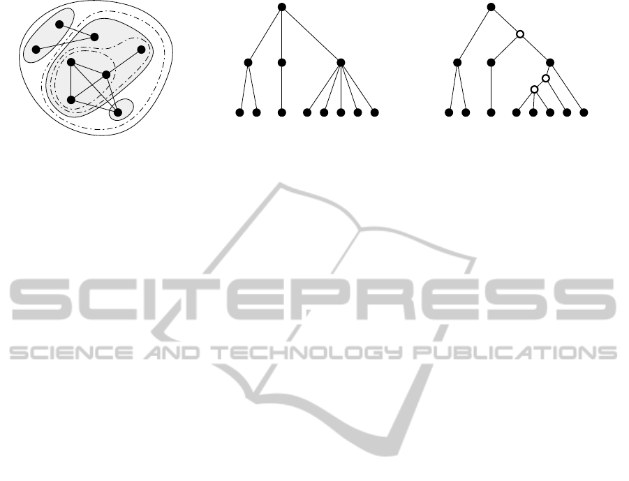
(a) Clustered Graph

a b c d e

f g

(b) Input Cluster Tree

a b c d e

f g

Figure 2: Example of a clustered graph (a) with cluster tree (b). The extended cluster tree (c) contains dummy nodes deter-

mined by betweenness based clustering. Dashed shapes in (a) depict the clusters representing these dummy nodes.

method is applied to the input, and thus the clusters

are consistent with the placement algorithm, nodes

that are well connected are placed close to each other,

while nodes with higher graph theoretic distance are

located in different subtrees. Before we present two

improvements, we sketch the outline of the original

method. First, the input graph is clustered using the

algorithm of (Girvan and Newman, 2002) to obtain

a cluster hierarchy with the aforementioned proper-

ties. Then a tree mapping approach called fat polygon

partitioning, based on (de Berg et al., 2010), is used.

The nodes are placed inside their partition that form a

nested structure of convex polygons representing the

hierarchy. The layout is then transformed into a trian-

gle mesh by applying a Delaunay triangulation. This

mesh serves both as a basis for drawing a topographic

map and as a routing network for edge bundling. For

more details, see (Gronemann and J

unger, 2012).

In the following we present two improvements

of the original method. First, we suggest to extend

the input hierarchy by adding virtual clusters with-

out changing the nested structure of the input. These

new clusters help to place highly connected groups of

nodes together. Second, the fat polygon partitioning is

modiﬁed to optimize edge length and to place clusters

based on an arbitrary edge set, while still generating

good polygons. The goal is to make the tree map al-

gorithm aware of the edges and exploit the degrees of

freedom offered by the input hierarchy and the poly-

gon partitioning. Finally, we evaluate the modiﬁca-

tions based on the instances of our application area.

4.1 Extending the Input Hierarchy

The inner nodes of the scaffold tree usually contain

many children. In this case the fat polygon partition

must create a binary subtree for the subdivision pro-

cedure. However, since the provided input hierarchy

is not edge-aware, the subdivision procedure may re-

sult in edge clutter. This is due to the fact that highly

connected child clusters are placed in distant subtrees.

In order to solve this problem, we use edge between-

ness clustering to extend the input hierarchy. The al-

gorithm proposed in (Girvan and Newman, 2002) is

rather simple. For all edges, the betweenness score

is calculated and the edges with the highest score are

removed. This procedure is repeated until the graph

becomes disconnected. The connected components

serve as clusters on which the method recurses.

This method can easily be adapted to work on an

existing hierarchy. We traverse the input hierarchy

top-down. For each cluster C with children C

,...,C

n > 2, we construct a graph G(C) induced by the

underlying edge set E and the children of C. Let

V (C

) denote the graph nodes contained in the subtree

rooted at C

. Let E(C

) = E ∩(V (C

) ×V (C

)) de-

note the edges having one end point in C

and the other

in C

. The obvious way to obtain the inter-cluster

edge weights w(C

) is to sum up the ‘cluster-

parallel’ edge weights according to

w(C

) =

∑

e∈E(C

)

w(e).

The original algorithm is then used to obtain a hierar-

chy for this graph, which we can insert into the exist-

ing subtree. The leaves of the obtained hierarchy cor-

respond to the children of the cluster node C, which

can be replaced by the root of the hierarchy.

In Figure 2 a small example is displayed. The

dashed shapes are the newly inserted clusters after the

algorithm has decomposed as much as possible with-

out violating the nested structure of the input hierar-

chy. The newly created clusters are used as “ghost

clusters”, which are not visible on the ﬁnal map. Their

only purpose is to group tightly connected compo-

nents together. In case that the result is not a bi-

nary tree, the transformation used in (Gronemann and

unger, 2012) is applied. Notice that the extended hi-

erarchy is based on intra-cluster adjacency only and

does not take external edges into account. This issue

is addressed in the following section.

IVAPP2013-InternationalConferenceonInformationVisualizationTheoryandApplications

518

(a) (b)

(c)

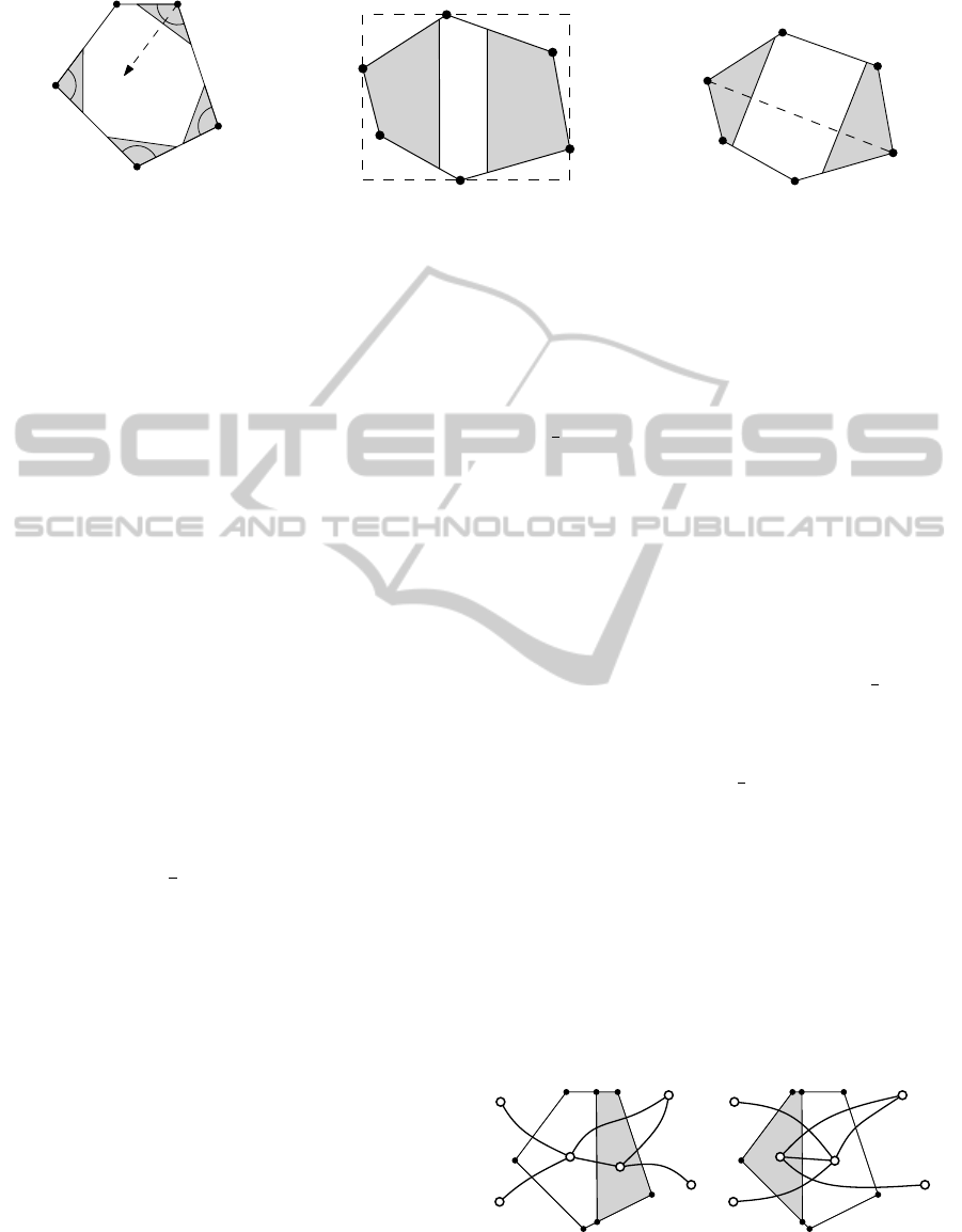
Figure 3: Enumeration of allowed cuts. In (a) we only want to cut off a small part of the polygon. The two choices when

choosing an axis-aligned cut and a cut perpendicular to the diameter deﬁned by v

are shown in (b) and (c), respectively.

4.2 Edge-aware Polygon Partitioning

In this section we investigate the degrees of freedom

of the polygon partitioning and how to exploit them

to minimize the length of edges between clusters.

A tree map based on fat polygon partitioning fol-

lows the same principle as most tree map algorithms.

The idea is to recursively subdivide a convex polygon

in order to obtain a nested structure of polygons repre-

senting the cluster tree. Starting with the root which

represents the boundary polygon the algorithm pro-

ceeds in a top-down manner: At each cluster node,

the associated polygon is split into two convex sub-

polygons which represent the subtrees rooted at the

two children. The cutting line is chosen, such that the

area of the subpolygons is proportional to the number

of leaves in the corresponding subtrees. We place the

graph nodes, i.e., the leaves of the tree, in the centroid

of the associated polygon computed by the partition-

ing.

The basic problem in the individual steps of the

partitioning algorithm can be summarized as follows:

We are given a convex polygon P with k vertices and

a parameter 0 < a ≤

, where a is the fraction of the

area we require for the smaller child. Let area(P) de-

note the area of P and diam(P) its diameter, i.e., the

maximum distance between two vertices of P. We

want to ﬁnd a direction for a cutting line that par-

titions P into two subpolygons P

and P

, such that

area(P

) = a ·area(P) and area(P

) = (1 −a)·area(P).

When given a cut direction, we choose the orienta-

tion of the cutting line perpendicular to this direc-

tion. In general ﬁnding such a cut is easy for a con-

vex polygon. However, an advantageous character-

istic of the greedy algorithm proposed in (de Berg

et al., 2010) is that it yields polygons with bounded

aspect ratios, where the aspect ratio is deﬁned as

asp(P) = diam(P)

/area(P). We want to preserve this

property without unnecessarily restricting the number

of allowed cuts.

In (de Berg et al., 2010) two main cases are dis-

tinguished: In the ﬁrst case, when we want to cut

off a small piece, that is when a ≤ 1/k

, the bisector

at the vertex with the smallest interior angle is taken

as the cut direction. However, the guarantee of the

small aspect ratio only relies on the fact that the small-

est interior angle of a convex polygon is bounded by

π·(1−

) (de Berg et al., 2010). Thus, we are allowed

to choose any other bisector as long as the interior an-

gle at the corresponding vertex is small enough. In

Figure 3(a) an example is given, where we are allowed

to choose every bisector, except the one at v

, which

is not small enough.

In the second case, when a > 1/k

, the aspect ratio

of the boundary polygon must be considered. When

P has a good aspect ratio, i.e., asp(P) ≤ k

, we are

allowed to choose any direction for a cut (de Berg

et al., 2010). In this case and when a >

holds,

our implementation chooses an axis-aligned cut nor-

mal to the longest side of the bounding rectangle for

aesthetic reasons, see Figure 3(b). Otherwise, when

asp(P) > k

or 1/k

< a ≤

holds, we choose the

direction of the line representing the diameter of the

polygon. This is the line that connects any two ver-

tices of P with maximum distance to each other, cf.

Figure 3(c).

The key idea is to enumerate all allowed cuts for

a given polygon and a parameter a in each step of the

partitioning procedure and to take the one that min-

imizes the edge length. That is, we try to place the

polygon of a child cluster in the direction of clusters

to which it is highly connected. Figure 4 illustrates

(a) (b)

Figure 4: Example for two possible partitions of a polygon

with adjacencies to external clusters. In (a) the total edge

length is less compared to the partition in (b).

MolMap-VisualizingMoleculeLibrariesasTopographicMaps

519

d, e,

f, g

(a) Initial situation

(b) Unbalanced reﬁnement

Figure 5: Example of layouts obtained for different reﬁnement strategies.

the idea. We will apply this procedure in a top down

manner to obtain a partitioning that is optimized for

edge length. However, there is no accurate informa-

tion available as to where these adjacent clusters are

located because the corresponding polygon has not

been computed yet. Therefore, we propose a heuristic

to decide which cut to use based on the partial knowl-

edge of the surrounding clusters.

The available information on node positions de-

pends on the current state of the subdivision pro-

cess. While the cluster tree is typically traversed in a

depth-ﬁrst fashion, we propose a different procedure

to achieve a more balanced level of reﬁnement: The

subdivision process always splits the polygon cover-

ing the larger area ﬁrst. We keep all cluster nodes

whose polygons still have to be partitioned in a pri-

ority queue Q ordered by area requirement. These

nodes, together with the leaves that have been pro-

cessed, form a layer L of nodes with associated poly-

gons that we call active. The polygons of all active

nodes cover the entire boundary polygon and realize

the preliminary layout on which the selection of an

allowed cut is based.

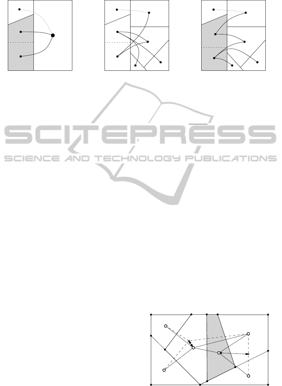
Figure 5 exempliﬁes the inﬂuence of the reﬁne-

ment order. When partitioning the gray polygon con-

taining a and b in Figure 5(a) there is no accurate

information available on the positions of d,e, f ,g.

Therefore, the polygon of a is placed in the middle

since minimizing the distance representing the length

of three inter-cluster edges is prioritized. The result

of this bad decision is displayed in Figure 5(b). When

polygons are partitioned in order of decreasing size

the information on neighboring polygons is more ac-

curate. This typically results in a better ﬁnal layout.

Figure 5(c) shows the cut that would be chosen after

the large right polygon has been reﬁned.

We introduce additional notation to precisely de-

ﬁne the criterion we use to assess the potential of a

cut to minimize edge lengths. Let C be a node of the

cluster tree. We use ctr(C) to refer to the centroid of

the associated polygon; awc(C) denotes the average

weighted center of the centroids of active polygons

adjacent to C weighted by inter-cluster edges, i.e.,

awc(C) =

w(C,L)

∑

P∈L

ctr(P) · w(C, P),

where w(C,L) =

∑

P∈L

w(C,P). The value of awc(C)

can be considered as the preferred location of (the

centroid of) the polygon associated with C.

Consider an active node C ∈ Q with children C

and C

. Each allowed cut assigns a subpolygon to the

two children, cf. Figure 3. The idea is to choose the

cut that minimizes the distance between the centroids

of the subpolygons and their preferred positions ac-

cording to the average weighted center. We deﬁne

the distance between the two points associated with a

node C as

dist(C) =



awc(C) −ctr(C)

if w(C,L) 6= 0,

0 otherwise.

Note that in the second case there are no edges leav-

ing the cluster C and the position of the polygon has

no effect on edge lengths. We choose the cut that min-

imizes

∑

i∈{1,2}

dist(C

) · w(C

,L), (1)

where the factor w(C

,L) reﬂects the impact of the in-

dividual children. Figure 6 illustrates the method for

a given cut.

awc(A)

awc(B)

ctr(B)

ctr(A)

Figure 6: Edge-aware cut selection

IVAPP2013-InternationalConferenceonInformationVisualizationTheoryandApplications

520

0.1

0.2

0.3

0.4

0.5

0.6

0.7

1.0 1.5 2.0 4.0 8.0

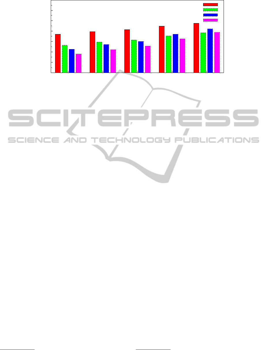
Average Weighted Edge Length

Density

Input Hierarchy

Edge-aware FPP + Input Hierarchy

Extended Hierarchy

Edge-aware FPP + Extended Hierarchy

Figure 7: Comparison of the average weighted edge length.

Putting all the above steps together, we can outline

the algorithm: We start with the root of the tree, assign

it the boundary polygon given as input and add it to

Q. Then we repeat the following steps until all leaves

have been processed.

1. Pop a node C with its boundary polygon P from

the queue Q.

2. If C is a leaf, add it to the active nodes and go to

the ﬁrst step, otherwise C must be partitioned.

3. Compute the fraction a of the area required for the

smaller child of C and check which case applies

based on a and P.

4. Enumerate all allowed cuts and choose the cut that

minimizes Equation (1).

5. Enqueue the two children in Q.

Notice that neither C nor its children are active during

the cut enumeration phase.

5 RESULTS & APPLICATION

In this section, we report on an experimental evalu-

ation of the proposed techniques to minimize edge

length and introduce several domain-speciﬁc exten-

sions.

5.1 Evaluation of Edge Length

In order to determine the effect on the layout, we

tested our approach on real-world datasets. The

instances were derived from a publicly available

pyruvate kinase high-throughput screening dataset

which has previously been used in (Wetzel et al.,

Available from PubChem BioAssay, AID 361

2009) and consists of 51, 415 compounds. We gener-

ated 20 subsets by randomly selecting 200, 400, 600

and 800 compounds, respectively. For each subset

we created clustered graphs according to the graph

model described in Section 3 with varying densities

by selecting suitable threshold parameters. We report

the average weighted edge length of these instances

drawn in the unit square. Figure 7 displays the re-

sults for different densities. It is clearly visible that

the two presented approaches affect the edge length

in a positive way. As expected, the effect is less when

the density increases. Interestingly, the changes made

to the fat polygon partitioning are signiﬁcant even for

higher densities, unlike the extension of the cluster

hierarchy. The latter performs well on the sparse in-

stances, while the result is slightly worse for the high-

est density in comparison to the edge-aware fat poly-

gon partitioning. The runtime

for the largest instance

with |V | = 800 and |E| = 6400 is about 7s for the clus-

ter extension and 0.6s for the edge-aware fat polygon

partitioning.

Figure 8 shows an example which illustrates the

effectiveness of the proposed techniques. Note that

in Figure 8(a) there are several long edges, some of

which even cross the entire drawing area connecting

nodes in the bottom left corner (cluster A) to nodes

in the top right corner (cluster E). In such cases edges

are bundled to avoid visual clutter. However, a down-

side of edge bundling is that individual edges become

difﬁcult to identify. In Figure 8(b) the same instance

is drawn using the proposed optimization techniques.

Here, the layout leads to short edges and individ-

ual connections are easily recognizable. Since highly

similar molecules are placed close to each other, this

drawing is also clearly preferable from the application

point of view.

Machine with Core i7 2.7 GHz and 8 GB RAM

MolMap-VisualizingMoleculeLibrariesasTopographicMaps

521

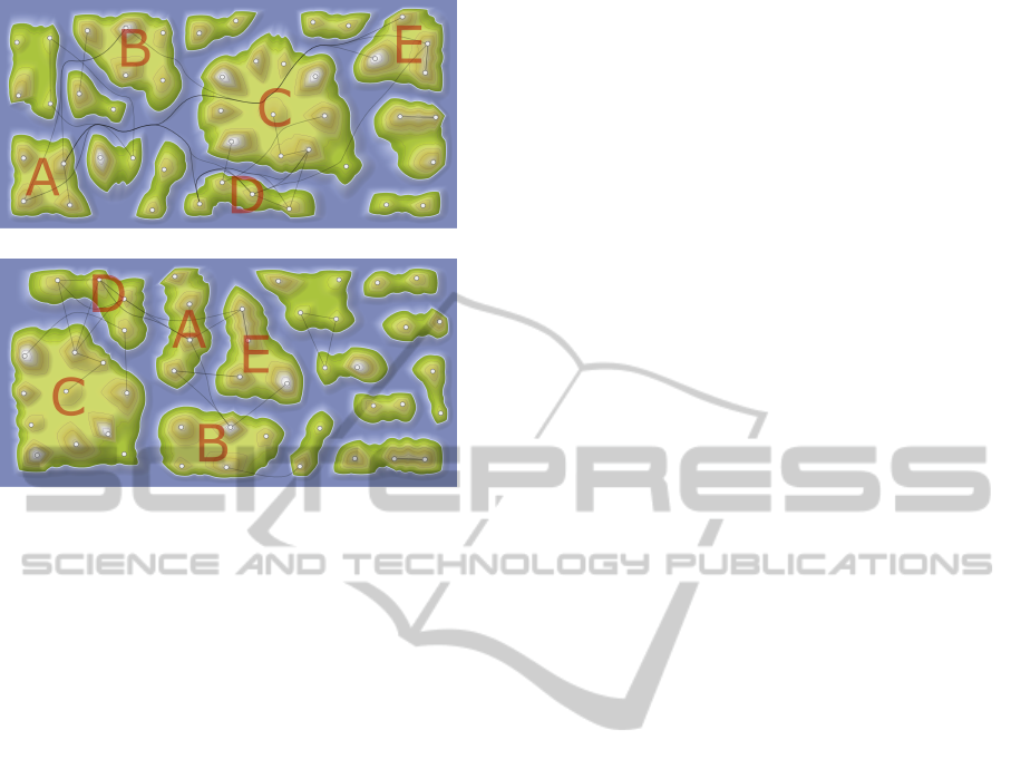
(a) Without improvements

(b) Extended hierarchy and edge-aware partitioning

Figure 8: Visual comparison of the layout generated by the

original approach (a) and the proposed method (b). Letters

indicate corresponding main clusters.

5.2 Representation of Chemical

Information

In this section we report on the application of our ap-

proach to a real-world dataset and describe several

extensions we incorporated to meet requirements of

the application area. To focus on relevant molecules

we ﬁltered the dataset used in Section 5.1 for active

compounds with AC

≤ 10µM and decreasing activ-

ity direction, which yields a dataset with 432 com-

pounds. From this subset we selected all molecules

associated with scaffold tree branches containing at

least 10 compounds. The threshold for the similarity

graph was set to t = 0.5. While our approach also

works smoothly with larger datasets, we decided to

use this small focused dataset consisting of 256 com-

pounds to provide screen shots.

The resulting topographic map is shown in Fig-

ure 9(a). Since the water level is chosen such that each

scaffold tree branch is represented by one island, this

overview directly conveys to what extent branches are

populated by compounds. With our approach the alti-

tude represents the number of rings compounds have

and whenever two molecules are located on the same

hill, they share a common scaffold (according to the

scaffold tree) whose number of rings is represented

by the elevation level of the hill. While edges often

connect molecules on the same islands, there are also

edges connecting molecules placed on different is-

lands (see, e.g., the central island on the left hand side

and the small island south-east) indicating the pres-

ence of highly similar molecules in different branches

of the scaffold tree. Placing these molecules near each

other helps to generate continuous regions of highly

similar molecules and is achieved by our heuristic ap-

proach. Furthermore, we support additional annota-

tions to speciﬁcally foster the application in drug dis-

covery.

5.2.1 Depiction of Structural Formulae

The most widely used representation of chemical

compounds are 2D depictions of their structure. To

allow a detailed investigation of structural relation-

ships, we support displaying structural formulae. Fig-

ure 9(b) shows a close-up view of a region of an is-

land. The shown molecules are placed on the same el-

evated plateau indicating their common two-ring scaf-

fold. The two molecules on the left hand side even

share a scaffold with three rings.

5.2.2 Mapping of Properties

While the topographic map is generated taking only

structural similarity of molecules into account, relat-

ing structural features with certain properties is of ut-

most importance in drug discovery. We support the

visualization of molecular properties by superimpos-

ing a heat map, faintly reminiscent of a temperature

related weather map. Figure 9(c) shows an example

where regions of highly active molecules are high-

lighted in red. The color gradient from red to green

represents decreasing activity. Regions not colored

are populated by less active molecules. The heat map

is generated by computing a Delaunay triangulation

and, similar to the topographic map, visualized using

color encoded levels based on the property values.

6 CONCLUSIONS & OUTLOOK

Organizing compound libraries by structural similar-

ity in a way that allows for intuitive navigation for

chemical tasks is challenging. We proposed a clus-

tered graph model and adapted a technique to draw

them as topographic maps. We have already received

some ﬁrst positive feedback from domain experts, and

the representation as topographic map has been well

accepted. However, a large-scale systematic evalua-

tion of the method based on a wide range of datasets

and different chemical workﬂows is out of the scope

of this article, but an important future task.

The goal to place similar molecules near each

other while respecting the cluster hierarchy leads to

IVAPP2013-InternationalConferenceonInformationVisualizationTheoryandApplications

522

(a) Real-world instance

(b) Close-up view (c) Superimposed heat map

Figure 9: Visualization of the real-world instance consisting of 256 molecules (a) and the same map with property annotations

(c). In (b) a close-up view of the region highlighted in red shows ﬁve molecules represented by structural formulae.

MolMap-VisualizingMoleculeLibrariesasTopographicMaps

523

the graph drawing problem to minimize edge length in

the known approach (Gronemann and J

unger, 2012).

To achieve this goal we proposed a heuristic that ex-

ploits the degrees of freedom in the polygon partition-

ing procedure in order to avoid long edges. The effec-

tiveness of the method has been demonstrated by an

experimental evaluation using real-world instances.

ACKNOWLEDGEMENTS

We would like to thank Claude Ostermann and

Philipp Thiel for their valuable feedback and for shar-

ing their chemical knowledge. Research was sup-

ported by the German Research Foundation (DFG),

priority programme “Algorithm Engineering” (SPP

1307).

REFERENCES

Bon, R. S. and Waldmann, H. (2010). Bioactivity-guided

navigation of chemical space. Acc. Chem. Res.,

43(8):1103–1114.

Brown, N. (2009). Chemoinformatics - an introduction for

computer scientists. ACM Comput. Surv., 41(2).

de Berg, M., Onak, K., and Sidiropoulos, A. (2010). Fat

polygonal partitions with applications to visualization

and embeddings. CoRR, abs/1009.1866.

Fabrikant, S. I., Montello, D. R., and Mark, D. M. (2010).

The natural landscape metaphor in information visu-

alization: The role of commonsense geomorphology.

J. Am. Soc. Inf. Sci. Technol., 61(2):253–270.

Fruchterman, T. M. J. and Reingold, E. M. (1991). Graph

drawing by force-directed placement. Softw., Pract.

Exper., 21(11):1129–1164.

Gansner, E. R., Hu, Y., and Kobourov, S. G. (2010). GMap:

Visualizing graphs and clusters as maps. In Paciﬁc

Visualization Symposium (PaciﬁcVis), pages 201–208.

IEEE.

Gansner, E. R., Hu, Y., Kobourov, S. G., and Volinsky, C.

(2009). Putting recommendations on the map: visual-

izing clusters and relations. In Proc. ACM Conference

on Recommender Systems, pages 345–348.

Girvan, M. and Newman, M. E. J. (2002). Community

structure in social and biological networks. Proc. of

the National Academy of Sciences, 99:7821–7826.

Gronemann, M. and J

unger, M. (2012). Drawing clustered

graphs as topographic maps. In 20th International

Symposium on Graph Drawing.

Herhaus, C., Karch, O., Bremm, S., and Rippmann,

F. (2009). MolWind - mapping molecule spaces

to geospatial worlds. Chemistry Central Journal,

3(Suppl 1):P32.

Huang, M. and Eades, P. (1998). A fully animated interac-

tive system for clustering and navigating huge graphs.

In Graph Drawing, volume 1547 of Lecture Notes in

Computer Science, pages 374–383. Springer.

Irwin, J. J. (2009). Staring off into chemical space. Nat.

Chem. Biol., 5(8):536–537.

Johnson, B. and Shneiderman, B. (1991). Tree-maps: a

space-ﬁlling approach to the visualization of hierar-

chical information structures. In Proc. of the 2nd Con-

ference on Visualization, pages 284–291.

Klein, K., Kriege, N., and Mutzel, P. (2012). Scaf-

fold Hunter – visual analysis of chemical compound

databases. In Proc. Int. Conf. on Computer Graphics

Theory and Applications and Int. Conf. on Informa-

tion Visualization Theory and Applications (GRAPP

& IVAPP), pages 626–635.

Lounkine, E., Wawer, M., Wassermann, A. M., and Bajo-

rath, J. (2010). SARANEA: a freely available program

to mine structure-activity and structure-selectivity re-

lationship information in compound data sets. J.

Chem. Inf. Model., 50(1):68–78.

Maggiora, G. M. and Shanmugasundaram, V. (2011).

Molecular similarity measures. Methods in Molecu-

lar Biology, 672:39–100.

Schuffenhauer, A., Ertl, P., Roggo, S., Wetzel, S., Koch,

M. A., and Waldmann, H. (2007). The scaffold tree

- visualization of the scaffold universe by hierarchical

scaffold classiﬁcation. J. Chem. Inf. Model., 47(1):47–

58.

Schuffenhauer, A. and Varin, T. (2011). Rule-based classi-

ﬁcation of chemical structures by scaffold. Molecular

Informatics, 30(8):646–664.

Schulz, H.-J. (2011). Treevis.net: A tree visualization ref-

erence. IEEE Computer Graphics and Applications,

31(6):11–15.

Steinbeck, C., Hoppe, C., Kuhn, S., Floris, M., Guha, R.,

and Willighagen, E. L. (2006). Recent developments

of the chemistry development kit (CDK) - an open-

source java library for chemo- and bioinformatics.

Current pharmaceutical design, 12(17):2111–2120.

Strobelt, H., Bertini, E., Braun, J., Deussen, O., Groth, U.,

Mayer, T. U., and Merhof, D. (2012). HiTSEE KN-

IME: a visualization tool for hit selection and analysis

in high-throughput screening experiments for the KN-

IME platform. BMC Bioinformatics, 13 Suppl 8:S4.

Sugiyama, K. and Misue, K. (1991). Visualization of struc-

tural information: Automatic drawing of compound

digraphs. IEEE Trans. SMC, 21(4):876–892.

Wawer, M., Peltason, L., Weskamp, N., Teckentrup, A.,

and Bajorath, J. (2008). Structure-activity relationship

anatomy by network-like similarity graphs and local

structure-activity relationship indices. J. Med. Chem.,

51(19):6075–6084.

Wetzel, S., Klein, K., Renner, S., Rauh, D., Oprea, T. I.,

Mutzel, P., and Waldmann, H. (2009). Interactive ex-

ploration of chemical space with Scaffold Hunter. Na-

ture Chemical Biology, 5(8):581–583.

IVAPP2013-InternationalConferenceonInformationVisualizationTheoryandApplications

524