
Measuring Linearity of Curves
Jovi
ˇ
sa
ˇ
Zuni
´
c
1
, Jovanka Pantovi
´
c
2
and Paul L. Rosin
3
1
University of Exeter, Computer Science, Exeter EX4 4QF, U.K.
2
Faculty of Technical Sciences, University of Novi Sad, 21000 Novi Sad, Serbia
3
Cardiff University, School of Computer Science, Cardiff CF24 3AA, U.K.
Keywords:
Shape, Shape Descriptors, Curves, Linearity Measure, Image Processing.
Abstract:
In this paper we define a new linearity measure which can be applied to open curve segments. The new
measure ranges over the interval (0, 1], and produces the value 1 if and only if the measured line is a perfect
straight line segment. Also, the new linearity measure is invariant with respect to translations, rotations and
scaling transformations.
1 INTRODUCTION
Shape descriptors have been employed in many com-
puter vision and image processing tasks (e.g. im-
age retrieval, object classification, object recognition,
object identification, etc). Different mathematical
tools have been used to define the shape descrip-
tors: algebraic invariants (Hu, 1962), geometric ap-
proaches (
ˇ
Zuni
´
c et al., 2010), Fourier analysis (Bow-
man et al., 2001), morphological operations (Ruberto
and Dempster, 2000), integral transformations (Rahtu
et al., 2006), statistical methods (Melter et al., 1993),
fractal techniques (Imre, 2009), logic (Schweitzer and
Straach, 1998), multiscale approaches (Direkoglu and
Nixon, 2011), integral invariants (Manay et al., 2006),
etc. Generally speaking, shape descriptors can be
classified into two groups: area based descriptors and
boundary based ones. Area based descriptors are
more robust (i.e. less sensitive to noise or shape defor-
mations) while boundary based descriptors are more
sensitive. A preference for either type of descriptor
depends on the application performed and the data
available. For example low quality data would re-
quire robust descriptors (i.e. area based ones) while
high precision tasks would require more sensitive de-
scriptors (i.e. boundary based ones). In the litera-
ture so far, more attention has been paid to the area
based descriptors, not only because of their robust-
ness but also because they are easier to be efficiently
estimated when working with discrete data. Due to
the recent proliferation of image verification, identi-
fication and recognition systems there is a strong de-
mand for shape properties that can be derived from
their boundaries (Manay et al., 2006; Mio et al., 2007;
Stojmenovi
´
c and
ˇ
Zuni
´
c, 2008). It is worth mentioning
that some objects, like human signatures for example,
are linear by their nature and area based descriptors
cannot be used for their analysis.
In this paper we deal with linearity measures that
should indicate the degree to which an open curve
segment differs from a perfect straight line segment.
Several linearity measures for curve segments are al-
ready considered in the literature (Gautama et al.,
2004; Gautama et al., 2003; Stojmenovi
´
c et al., 2008;
ˇ
Zuni
´
c and Rosin, 2011).
Perhaps the simplest way to define the linearity
measure of an open curve segment is to consider the
ratio between the length of the curve considered and
the distance between its end points. This is a natural
and simple definition which is also called the straight-
ness index (Benhamou, 2004). It satisfies the follow-
ing basic requirements for a linearity measure of open
curve segments.
• The straightness index varies through the interval
[0, 1];
• The straightness index equals 1 only for straight
line segments;
• The straightness index is invariant with respect to
translation, rotation and scaling transformation on
a curve considered.
Also, the straightness index is simple to compute and
its behavior can be clearly predicted, i.e. we can see
easily which curves have the same linearities, mea-
sured by the straightness index. It is obvious that
388
Žuni
´
c J., Pantovi
´
c J. and L. Rosin P. (2013).
Measuring Linearity of Curves.
In Proceedings of the 2nd International Conference on Pattern Recognition Applications and Methods, pages 388-395
DOI: 10.5220/0004267603880395
Copyright
c
SciTePress

those curves whose end points and the length coin-
cide, have the same straightness index. But the diver-
sity of such curves is huge and the straightness index
cannot distinguish among them, which could be a big
drawback in certain applications. Some illustrations
using simple polygonal curves are shown in Fig. 1.
Figure 1: Five displayed curves (solid lines) have different
linearities measured by L(C ). The straightness index has
the same value for all three curves.
In this paper we define a new linearity measure
L(C ) for open curve segments. The new measure sat-
isfies the basic requirements (listed above) which are
expected to be satisfied for any curve linearity mea-
sure. Since it considers the distance of the end points
of the curve to the centroid of the curve, the new mea-
sure is also easy to compute. The fact that it uses the
curve centroids implies that it takes into account a rel-
ative distribution of the curve points.
The paper is organized as follows. Section 2 gives
basic definitions and denotation. The new linearity
measure for planar open curve segments is in Section
3. Several experiments which illustrate the behavior
and the classification power of the new linearity mea-
sure are provided in Section 4. Concluding remarks
are in Section 5.
2 DEFINITIONS
AND DENOTATIONS
Without loss of generality, throughout the paper, it
will be assumed (even if not mentioned) that every
curve C has length equal to 1 and is given in an arc-
length parametrization. I.e., planar curve segment C
is represented as:
x = x(s), y = y(s), where s ∈ [0, 1].
The parameter s measures the distance of the point
(x(s), y(s)) from the curve start point (x(0), y(0)),
along the curve C .
The centroid of a given planar curve C will be de-
noted by (x
C
, y
C
) and computed as
(x
C
, y
C
) =
Z
C
x(s) ds,
Z
C
y(s) ds
. (1)
Taking into account that the length of C is as-
sumed to be equal to 1, we can see that the coordi-
nates of the curve centroid, as defined in (1), are the
average values of the curve points.
As usual,
d
2
(A, B) =
q
(x − u)
2
+ (y − v)
2
will denote the Euclidean distance between the points
A = (x, y) and B = (u, v).
As mentioned, we introduce a new linearity mea-
sure L(C ) which assigns a number from the interval
(0, 1]. The curve C is assumed to have the length 1.
More precisely, any appearing curve will be scaled by
the factor which equals the length of it before the pro-
cessing. So, an arbitrary curve C would be replaced
with the curve C defined by
C =
1
R
C
a
ds
· C
a
=
x
R
C
a
ds
,
y
R
C
a
ds
| (x, y) ∈ C
a
Shape descriptors/measures are very useful for
discrimination among the objects – in this case open
curve segments. Usually the shape descriptors have a
clear geometric meaning and, consequently, the shape
measures assigned to such descriptors have a pre-
dictable behavior. This is an advantage because the
suitability of a certain measure to a particular shape-
based task (object matching, object classification, etc)
can be predicted to some extent. On the other hand, a
shape measure assigns to each object (here curve seg-
ment) a single number. In order to increase the perfor-
mance of shape based tasks, a common approach is to
assign a graph (instead of a number) to each object.
E.g. such approaches define shape signature descrip-
tors, which are also ‘graph’ representations of planar
shapes, often used in shape analysis tasks (El-ghazal
et al., 2009; Zhang and Lu, 2005), but they differ from
the idea used here.
We will apply a similar idea here as well. To
compare objects considered we use linearity plots to
provide more information than a single linearity mea-
surement. The idea is to compute linearity incremen-
tally, i.e. to compute linearity of sub-segments of C
determined by the start point of C and another point
which moves along the curve C from the beginning
of to the end of C. The linearity plot P(C ), associated
with the given curve C is formally defined as follows.
Definition 1. Let C be a curve given in an arc-length
parametrization: x = x(s), y = y(s), and s ∈ [0, 1]. Let
A(s) be the part of the curve C bounded by the start-
ing point (x(0), y(0)) and by the point (x(s), y(s)) ∈ C .
Then, for a linearity measure L, the linearity plot
P(C ) is defined by:
P(C ) = {(s, L(A(s)) | s ∈ [0, 1]}. (2)
We also will use the reverse linearity plot P
rev
(C )
defined as:
P
rev
(C ) = {(s, L(A
rev
(1 − s)) | s ∈ [0, 1]}, (3)
MeasuringLinearityofCurves
389

where A
rev
(1 − s) is the segment of the curve C de-
termined by the end point (x(1), y(1)) of C and the
point which moves from the end point of C , to the
start point of C , along the curve C . In other words,
P
rev
(C ) is the linearity plot of the curve C
0
which co-
incides with the curve C but the start (end) point of
C is the end (start) point of C
0
. A parametrization of
C
0
can be obtained by replacing the parameter s, in
the parametrization of C , by a new parameter s
0
such
that s
0
= 1 − s. Obviously such a defined s
0
measures
the distance of the point (x(s
0
), y(s
0
)) from the starting
point (x(s
0
= 0), y(s
0
= 0)) of C
0
along the curve C
0
,
as s
0
varies through the interval [0, 1].
3 NEW LINEARITY MEASURE
FOR OPEN CURVE SEGMENTS
In this section we introduce a new linearity measure
for open planar curve segments.
We start with the following theorem which says
that amongst all curves having the same length,
straight line segments have the largest sum of dis-
tances between the curve end points to the curve cen-
troid. This result will be exploited to define the new
linearity measure for open curve segments.
Theorem 1. Let C be an open curve segment given in
an arc-length parametrization x = x(s), y = y(s), and
s ∈ [0, 1]. The following statements hold:
(a) The sum of distances of the end points (x(0), y(0))
and (x(1), y(1)) from the centroid (x
C
, y
C
) of the
curve C is bounded from above by 1, i.e.:
d
2
((x(0), y(0)), (x
C
, y
C
))
+ d
2
((x(1), y(1)), (x
C
, y
C
))
≤ 1. (4)
(b) The upper bound established by the previous item
is reached by the straight line segment and, con-
sequently, cannot be improved.
Proof. Let C be a curve given in an arc-length
parametrization: x = x(s) and y = y(s), with s ∈ [0, 1],
and let S = (x(0), y(0)) and E = (x(1), y(1)) be the
end points of C . We can assume, without loss of gen-
erality, that the curve segment C is positioned such
that
• the end points S and E belong to the x-axis (i.e.
y(0) = y(1) = 0), and
• S and E are symmetric with respect to the origin
(i.e. −x(0) = x(1)),
as illustrated in Fig. 2.
Furthermore, let
E = {X = (x, y) | d
2
(X, S) + d
2
(X, E) = 1}
be an ellipse which consists of points whose sum of
distances to the points S and E is equal 1. Now, we
prove (a) in two steps.
(i) First, we prove that the curve C and the ellipse E
do not have more than one intersection point (i.e.
C belongs to the closed region bounded by E).
This will be proven by a contradiction. So, let
us assume the contrary, that C intersects E at k
(k ≥ 2) points:
(x(s
1
), y(s
1
)), (x(s
2
), y(s
2
)), ..., (x(s
k
), y(s
k
)),
where 0 < s
1
< s
2
< . . . < s
k
< 1. Let A =
(x(s
1
), y(s
1
)) and B = (x(s
k
), y(s
k
)). Since the
sum of the lengths of the straight line segments
[SA] and [AE] is equal to 1, the length of the poly-
line SABE is, by the triangle inequality, bigger
than 1. Since the length of the arc
c
SA (along the
curve C ) is not smaller than the length of the edge
[SA], the length of the arc
c
AB (along the curve
C ) is not smaller than the length of the straight
line segment [AB], and the length of the arc
c
BE
(along the curve C ) is not smaller than the length
of the straight line segment [BE], we deduce that
the curve C has length bigger than 1, which is a
contradiction. A more formal derivation of the
contradiction 1 < 1 is
1 = d
2
(S, A) + d
2
(A, E)
< d
2
(S, A) + d
2
(A, B) + d
2
(B, E)
≤
Z
c
SA
ds +
Z
c
AB
ds +
Z
c
BE
ds =
Z
C
ds
= 1. (5)
So, C and E do not have more than one intersec-
tion point, implying that C lies in the closed re-
gion bounded by E.
(ii) Second, we prove that the centroid of C does not
lie outside of E.
The proof follows easily:
– the convex hull CH(C ) of C is the smallest con-
vex set which includes C and, consequently, is
a subset of the region bounded by E;
– The centroid of C lies in the convex hull CH(C )
of C because it belongs to every half plane
which includes C (the intersection of such half
planes is actually the convex hull of C (see
(Valentine, 1964)));
– the two items above give the required:
(x
C
, y
C
) ∈ CH(C ) ⊂ region bounded by E.
ICPRAM2013-InternationalConferenceonPatternRecognitionApplicationsandMethods
390
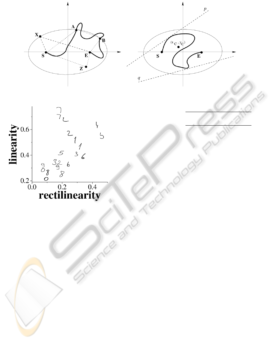
Figure 2: Denotations in the proof of Theorem 1 are illustrated above.
Figure 3: Handwritten digits ordered by linearity and recti-
linearity.
Finally, since the centroid of C does not lie
outside E , the sum of the distances of the centroid
(x
C
, y
C
) of C to the points S and E may not be bigger
than 1, i.e.
d
2
((x(0), y(0)), (x
C
, y
C
)) + d
2
((x(1), y(1)), (x
C
, y
C
))
= d
2
(S, (x
C
, y
C
)) + d
2
(E, (x
C
, y
C
))
≤ 1.
This establishes (a).
To prove (b) it is enough to notice that if C is a
straight line segment of length 1, then the sum of its
end points to the centroid of C is 1.
Now, motivated by the results of Theorem 1, we
give the following definition for a new linearity mea-
sure L(C ) for open curve segments.
Definition 2. Let C be an open curve segment. Then,
the linearity measure L(C ) of C is defined as the sum
of distances between the centroid (x
C
, y
C
) of C and
the end points of C . I.e.:
L(C ) =
q
(x(0) − x
C
)
2
+ (y(0) − y
C
)
2
+
q
(x(1) − x
C
)
2
+ (y(1) − y
C
)
2
where x = x(s), y = y(s), s ∈ [0, 1] is an arc-length
representation of C .
The following theorem summarizes desirable
properties of L(C ).
Theorem 2. The linearity measure L(C ) has the fol-
lowing properties:
(i) L(C ) ∈ (0, 1], for all open curve segments C ;
(ii) L(C ) = 1 ⇔ C is a straight line segment;
(iii) L(C ) is invariant with respect to the similarity
transformations.
Proof. Item (i) is a direct consequences of Theorem
1.
To prove (ii) we will use the same notations as in
the proof of Theorem 1 and give a proof by contradic-
tion. So, let assume the following:
– the curve C differs from a straight line segment, and
– the sum of distances between the end points, and the
centroid of C is 1.
Since C is not a straight line segment, then d
2
(S, E) <
1, and the centroid (x
C
, y
C
) lies on the ellipse E =
{X = (x, y) | d
2
(X, S) + d
2
(X, E) = 1}. Further, it
would mean that there are points of the curve C be-
longing to both hyperplanes determined by the tan-
gent on the ellipse E passing through the centroid of
C . This would contradict the fact that C and E do
not have more than one intersection point (what was
proven as a part of the proof of Theorem 1).
To prove item (iii) it is enough to notice that trans-
lations and rotations do not change the distance be-
tween the centroid and the end points. Since we as-
sume that C is represented by using an arc-length
parametrization: x = x(s), y = y(s), with the parame-
ter s varying through [0,1], the new linearity measure
MeasuringLinearityofCurves
391
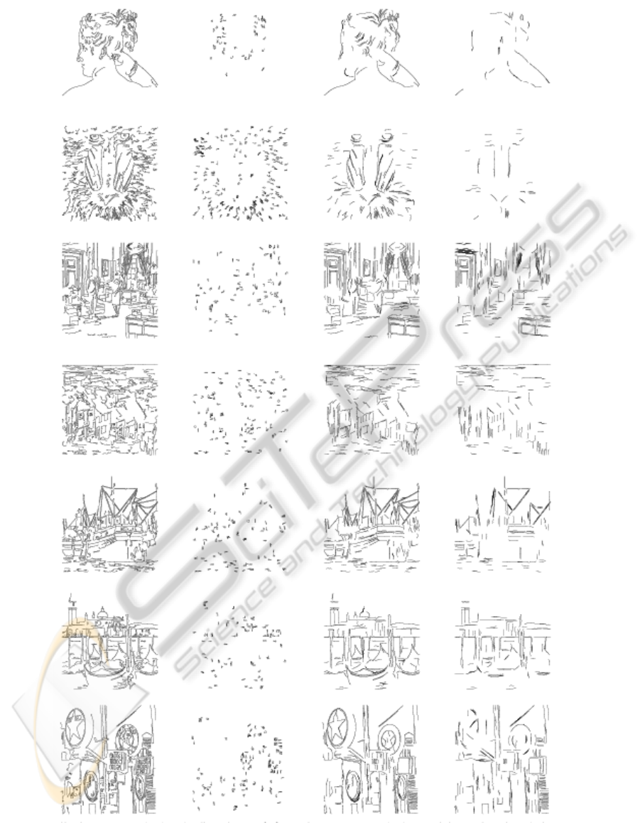
Figure 4: Filtering connected edges by linearity. Left/first column: connected edges (minimum length: 25 pixels); second
column: sections of curve with L (C ) < 0.5; third column: sections of curve with L(C ) > 0.9; fourth column: sections of
curve with L(C) > 0.95.
ICPRAM2013-InternationalConferenceonPatternRecognitionApplicationsandMethods
392
L(C ) is invariant with respect to scaling transforma-
tions as well.
4 EXPERIMENTS
In this section we provide several experiments in or-
der to illustrate the behavior and efficiency of the lin-
earity measure introduced here.
First Experiment: Behavior Illustration. To
demonstrate how various shapes produce a range of
linearity values, figure 3 shows the first two samples
of each handwritten digit (0–9) from the training set
captured by Alimo
˘
glu and Alpaydin (Alimo
˘
glu and
Alpaydin, 2001) plotted in a 2D feature space of lin-
earity L(C ) versus rectilinearity R
1
(C ) (
ˇ
Zuni
´
c and
Rosin, 2003).
Despite the variability of hand writing, most pairs
of the same digit are reasonably clustered. The major
separations occur for:
– “2” since only one instance has a loop in the mid-
dle;
– “4” since the instance next to the pair of “7”s is
missing the vertical stroke;
– “5” since the uppermost right instance is missing
the horizontal stroke.
Second Experiment: Filtering Edges. Figure 4
shows the application of the linearity to filtering
edges. The edges were extracted from the images us-
ing the Canny detector (Canny, 1986), connected into
curves, and then thresholded according to total edge
magnitude and length (Rosin, 1997). Linearity was
measured in local sections of curve of length 25, and
sections above (or below) a linearity threshold were
retained. It can be seen that retaining sections of curve
with L(C ) < 0.5 finds small noisy or corner sec-
tions. Keeping sections of curve with L(C ) > 0.9 or
L(C ) > 0.95 identifies most of the significant struc-
tures in the image.
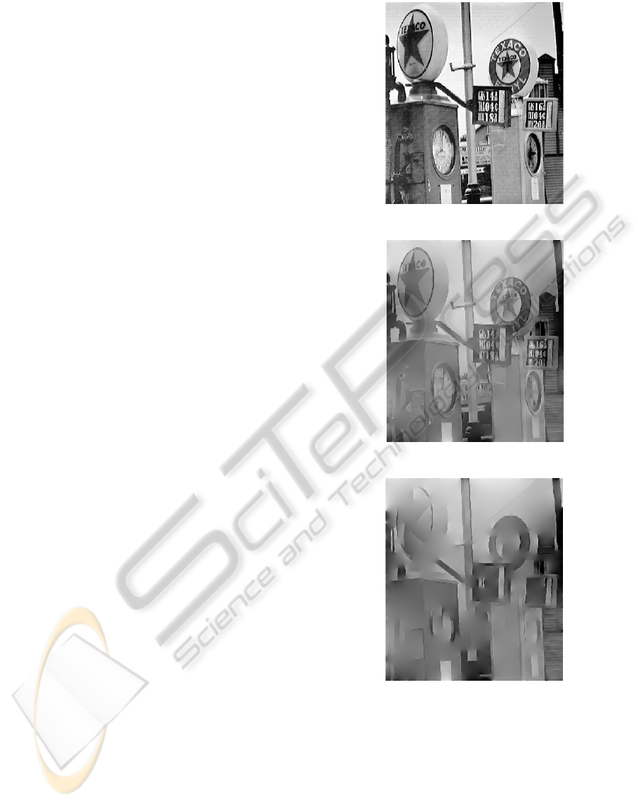
Experiments are also shown in which Poisson im-
age reconstruction is performed from the image gradi-
ents (P
´
erez et al., 2003). In figure 5b all the connected
edges with minimum length of 25 pixels (shown at
the bottom of the first column in figure 4) are used
as a mask to eliminate all other edges before recon-
struction. Some fine detail is removed as expected
since small and weak edges have been removed in
the pre-processing stage. When linearity filtering is
applied, and only edges corresponding to sections of
curve with L(C ) > 0.95 are used (see bottom of the
(a)
(b)
(c)
Figure 5: Reconstructing the image from its filtered edges.
(a) original intensity image; (b) image reconstructed using
all connected edges (minimum length: 25 pixels); (c) image
reconstructed using sections of curve with L(C) > 0.95.
fourth column in figure 5) then the image reconstruc-
tion retains only regions that are locally linear struc-
tures (including sections of large circular objects).
Third Experiment: Signature Verification. For
the second application we use data from Munich and
MeasuringLinearityofCurves
393
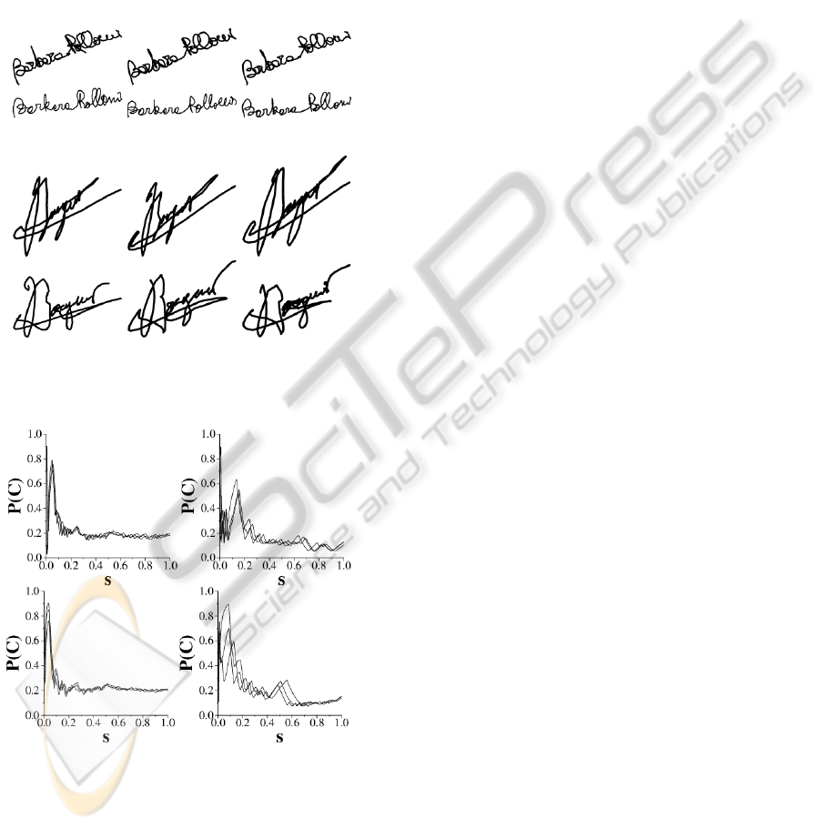
Perona (Munich and Perona, 2003) to perform signa-
ture verification. The data consists of pen trajectories
for 2911 genuine signatures taken from 112 subjects,
plus five forgers provided a total of 1061 forgeries
across all the subjects. Examples of corresponding
genuine and forged signatures are shown in Figure 6.
To compare signatures we use the linearity plots de-
fined by (2) and (3) to provide more information than
a single linearity measurement. Linearity plot exam-
ples are in figure 7.
Figure 6: Examples of genuine (first and third rows) and
forged (second and fourth rows) signatures.
Figure 7: Examples of linearity plots for the genuine sig-
natures (top row) and the forged signatures (bottom row) in
figure 6.
The quality of match between signatures C
1
and
C
2
is measured by the similarity between the linear-
ity plots P(C
1
) and P(C
2
). This similarity is measured
by the area bounded by the linearity plots P(C
1
) and
P(C
2
) and by the vertical lines s = 0 and s = 1. Fig-
ure 7 demonstrates the linearity plots for the signa-
tures shown in figure 6. The plots in the first (second
respectively) row contain the three genuine (forged
respectively) signatures from figure 6.
Nearest neighbour matching is then performed on
all the data using the leave-one-out strategy. Signature
verification is a two class (genuine or fake) problem.
Since the identity of the signature is already known,
the nearest neighbour matching is only applied to the
set of genuine and forged examples of the subject’s
signature. Computing linearity of the signatures us-
ing L (C ) produces 96.9% accuracy. This improves
the results obtained by using the linearity measure
defined in (
ˇ
Zuni
´
c and Rosin, 2011) which achieved
93.1% accuracy.
5 CONCLUSIONS
This paper has described a new shape descriptor L(C )
for computing the linearity of open curve segments.
It is both extremely simple to implement and efficient
to compute. In addition, it satisfies the basic require-
ments for a linearity measure:
• L(C ) is in the interval (0, 1];
• L(C ) equals 1 only for straight line segments;
• L(C ) is invariant with respect to translation, rota-
tion and scaling transformation on a curve consid-
ered.
Finally, experiments show the effectiveness of the
new linearity measure on a variety of tasks.
ACKNOWLEDGEMENTS
This work is partially supported by the Serbian Min-
istry of Science and Technology/project III44006.
J. Pantovi
´
c and J.
ˇ
Zuni
´
c are also with the Mathe-
matical Institute of the Serbian Academy of Sciences
and Arts, Belgrade.
REFERENCES
Alimo
˘
glu, F. and Alpaydin, E. (2001). Combining multiple
representations for pen-based handwritten digit recog-
nition. ELEKTRIK: Turkish Journal of Electrical En-
gineering and Computer Sciences, 9(1):1–12.
Benhamou, S. (2004). How to reliably estimate the tortu-
osity of an animals path: straightness, sinuosity, or
fractal dimension? Journal of Theoretical Biology,
229(2):209–220.
ICPRAM2013-InternationalConferenceonPatternRecognitionApplicationsandMethods
394

Bowman, E., Soga, K., and Drummond, T. (2001). Particle
shape characterisation using fourier descriptor analy-
sis. Geotechnique, 51(6):545–554.
Canny, J. (1986). A computational approach to edge de-
tection. IEEE Trans. on Patt. Anal. and Mach. Intell.,
8(6):679–698.
Direkoglu, C. and Nixon, M. (2011). Shape classifica-
tion via image-based multiscale description. Pattern
Recognition, 44(9):2134–2146.
El-ghazal, A., Basir, O., and Belkasim, S. (2009). Farthest
point distance: A new shape signature for Fourier de-
scriptors. Signal Processing: Image Communication,
24(7):572–586.
Gautama, T., Mandi
´
c, D., and Hull, M. V. (2004). A
novel method for determining the nature of time se-
ries. IEEE Transactions on Biomedical Engineering,
51(5):728–736.
Gautama, T., Mandi
´
c, D., and Hulle, M. V. (2003). Signal
nonlinearity in fMRI: A comparison between BOLD
and MION. IEEE Transactions on Medical Images,
22(5):636–644.
Hu, M. (1962). Visual pattern recognition by moment in-
variants. IRE Trans. Inf. Theory, 8(2):179–187.
Imre, A. (2009). Fractal dimension of time-indexed paths.
Applied Mathematics and Computation, 207(1):221–
229.
Manay, S., Cremers, D., Hong, B.-W., Yezzi, A., and
Soatto, S. (2006). Integral invariants for shape match-
ing. IEEE Trans. on Patt. Anal. and Mach. Intell.,
28(10):1602–1618.
Melter, R., Stojmenovi
´
c, I., and
ˇ
Zuni
´
c, J. (1993). A new
characterization of digital lines by least square fits.
Pattern Recognition Letters, 14(2):83–88.
Mio, W., Srivastava, A., and Joshi, S. (2007). On shape of
plane elastic curves. Int. Journal of Computer Vision,
73(3):307–324.
Munich, M. and Perona, P. (2003). Visual identification by
signature tracking. IEEE Trans. on Patt. Anal. and
Mach. Intell., 25(2):200–217.
P
´
erez, P., Gangnet, M., and Blake, A. (2003). Poisson im-
age editing. ACM Trans. Graph., 22(3):313–318.
Rahtu, E., Salo, M., and Heikkil
¨
a, J. (2006). A new convex-
ity measure based on a probabilistic interpretation of
images. IEEE Trans. on Patt. Anal. and Mach. Intell.,
28(9):1501–1512.
Rosin, P. (1997). Edges: saliency measures and auto-
matic thresholding. Machine Vision and Applications,
9(4):139–159.
Ruberto, C. D. and Dempster, A. (2000). Circularity mea-
sures based on mathematical morphology. Electronics
Letters, 36(20):1691–1693.
Schweitzer, H. and Straach, J. (1998). Utilizing moment
invariants and gr
¨
obner bases to reason about shapes.
Computational Intelligence, 14(4):461–474.
Stojmenovi
´
c, M., Nayak, A., and
ˇ
Zuni
´
c, J. (2008). Measur-
ing linearity of planar point sets. Pattern Recognition,
41(8):2503–2511.
Stojmenovi
´
c, M. and
ˇ
Zuni
´
c, J. (2008). Measuring elon-
gation from shape boundary. Journal Mathematical
Imaging and Vision, 30(1):73–85.
Valentine, F. (1964). Convex Sets. McGraw-Hill, New York.
ˇ
Zuni
´
c, J., Hirota, K., and Rosin, P. (2010). A Hu moment in-
variant as a shape circularity measure. Pattern Recog-
nition, 43(1):47–57.
ˇ
Zuni
´
c, J. and Rosin, P. (2003). Rectilinearity meaurements
for polygons. IEEE Trans. on Patt. Anal. and Mach.
Intell., 25(9):1193–3200.
ˇ
Zuni
´
c, J. and Rosin, P. (2011). Measuring linearity of
open planar curve segments. Image Vision Comput-
ing, 29(12):873–879.
Zhang, D. and Lu, G. (2005). Study and evaluation of dif-
ferent Fourier methods for image retrieval. Image and
Vision Computing, 23(1):3349.
MeasuringLinearityofCurves
395
