Probabilistic Evidence Accumulation for Clustering Ensembles
Andr
´
e Lourenc¸o
1,2
, Samuel Rota Bul
`
o
3
, Nicola Rebagliati
3
, Ana Fred
2
, M
´
ario Figueiredo
2
and Marcello Pelillo
3
1
Instituto Superior de Engenharia de Lisboa, Lisbon, Portugal
2
Instituto de Telecomunicac¸
˜
oes, Instituto Superior T
´
ecnico, Lisbon, Portugal
3
DAIS, Universit
`
a Ca’ Foscari Venezia, Venice, Italy
Keywords:
Clustering Algorithm, Clustering Ensembles, Probabilistic Modeling, Evidence Accumulation Clustering.
Abstract:
Ensemble clustering methods derive a consensus partition of a set of objects starting from the results of a
collection of base clustering algorithms forming the ensemble. Each partition in the ensemble provides a set of
pairwise observations of the co-occurrence of objects in a same cluster. The evidence accumulation clustering
paradigm uses these co-occurrence statistics to derive a similarity matrix, referred to as co-association matrix,
which is fed to a pairwise similarity clustering algorithm to obtain a final consensus clustering. The advantage
of this solution is the avoidance of the label correspondence problem, which affects other ensemble clustering
schemes. In this paper we derive a principled approach for the extraction of a consensus clustering from the
observations encoded in the co-association matrix. We introduce a probabilistic model for the co-association
matrix parameterized by the unknown assignments of objects to clusters, which are in turn estimated using
a maximum likelihood approach. Additionally, we propose a novel algorithm to carry out the parameter
estimation with convergence guarantees towards a local solution. Experiments on both synthetic and real
benchmark data show the effectiveness of the proposed approach.
1 INTRODUCTION
Clustering ensemble methods obtain consensus solu-
tions from the results of a set of base clustering al-
gorithms forming the ensemble. Several authors have
shown that these methods tend to reveal more robust
and stable cluster structures than the individual clus-
terings in the ensemble (Fred, 2001; Fred and Jain,
2002; Strehl and Ghosh, 2002). The leverage of an
ensemble of clusterings is considerably more difficult
than combining an ensemble of classifiers, due to the
correspondence problem between the cluster labels
produced by the different clustering algorithms. This
problem is made more serious if additionally cluster-
ings with different numbers of clusters are allowed in
the ensemble.
In (Fred, 2001; Fred and Jain, 2002; Fred and Jain,
2005; Strehl and Ghosh, 2002), the clustering ensem-
ble is summarized into a pair-wise co-association ma-
trix, where each entry counts the number of cluster-
ings in the ensemble in which a given pair of objects is
placed in the same cluster, thus sidestepping the clus-
ter label correspondence problem. This matrix, which
is regarded to as a similarty matrix, is then used to fe-
ed a pairwise similarity clustering algorithm to deliver
the final consensus clustering (Fred and Jain, 2005).
The drawback of this approach is that the information
about the very nature of the co-association matrix is
not properly exploited during the consensus cluster-
ing extraction.
A first work in the direction of finding a more
principled way of using the information in the co-
association matrix is (Rota Bul
`
o et al., 2010). There,
the problem of extracting a consensus partition was
formulated as a matrix factorization problem, under
probability simplex constraints on each column of
the factor matrix. Each of these columns can then
be interpreted as the multinomial distribution that ex-
presses the probabilities of each object being assigned
to each cluster. The drawback of that approach is that
the matrix factorization criterion is not supported on
any probabilistic estimation rationale.
In this paper we introduce a probabilistic model
for the co-association matrix, entitled PEACE - Prob-
abilistic Evidence Accumulation for Clustering En-
sembles, whose entries are regarded to as independent
observations of binomial random variables count-
ing the number of times two objects occur in a
58
Lourenço A., Rota Bulò S., Rebagliati N., Fred A., Figueiredo M. and Pelillo M. (2013).
Probabilistic Evidence Accumulation for Clustering Ensembles.
In Proceedings of the 2nd International Conference on Pattern Recognition Applications and Methods, pages 58-67
DOI: 10.5220/0004267900580067
Copyright
c
 SciTePress

same cluster. These random variables are indirectly
parametrized by the unknown assignments of objects
to clusters, which are in turn estimated by adopting a
maximum-likelihood approach. This translates into a
non-linear optimization problem, which is addressed
by means of a primal line-search procedure that guar-
antees to find a local solution. Experiments on real-
world datasets from the UCI machine learning repos-
itory, on text-data benchmark datasets as well as on
synthetic datasets show the effectiveness of the pro-
posed approach.
The remainder of the paper is organized as fol-
lows. In Section 2, we describe our probabilistic
model for the co-association matrix and the related
maximum-likelihood estimation of the unknown clus-
ter assignments. Section 3 is devoted to solving the
optimization problem arising for the unknown clus-
ter assignments estimation. Section 4 contextualizes
this model on related work. Finally, Section 5 reports
experimental results and Section 6 presents some con-
cluding remarks.
2 PROBABILISTIC MODEL
Let O = {1,...,n} be the indices of a set of objects to
be clustered into K classes and let E = {p
u
}
N
u=1
be a
clustering ensemble, i.e., a set of N clusterings (parti-
tions) obtained by different algorithms (e.g., different
parametrizations and/or initializations) on (possibly)
sub-sampled versions of the object set. Each cluster-
ing p
u
∈ E is a function p
u
: O
u
→ {1,...,K
u
}, where
O
u
⊆ O is a sub-sample of O used as input to the
uth clustering algorithm, and K
u
is the corresponding
number of clusters, which can be different on each
p
u
∈ E . Let Ω
i j
⊆ {1,...,N} denote the set of clus-
tering indices where both objects i and j have been
clustered, i.e. , (u ∈ Ω) ⇔

(i ∈O
u
) ∧( j ∈ O
u
)

, and
let N
i j
= |Ω
i j
| be its cardinality. The ensemble of
clusterings is summarized in the co-association ma-
trix C = [c
i j
] ∈ {0,..., N}
n×n
. Each entry c
i j
of this
matrix having i 6= j counts the number of times ob-
jects i and j are observed as clustered together in the
ensemble E , i.e.
c
i j
=
∑
l∈Ω
i j
[p
l
(i) = p
l
( j)]
where [·] is an indicator function returning 1 or 0
according to whether the condition given as argument
is true or false. Of course, c
i j
∈ {0,...,N
i j
}.
Our basic assumption is that each object has an
(unknown) probability of being assigned to each clus-
ter independently of other objects. We denote by y
i
=
(y
1i
,...,y
Ki
)
>
the probability distribution over the set
of class labels {1, .. ., K}, that is y
ki
= P[i ∈C
k
], where
C
k
denotes the subset of O that constitutes the kth
cluster. Of course, y
i
belongs to the probability sim-
plex ∆
K
= {x ∈R
K
+
:
∑
K
j=1
x
j
= 1}. Finally, we collect
all the y
i
’s in a K ×n matrix Y = [y
1
,...,y
n
] ∈ ∆
n
K
.
In our model, the probability that objects i and j
are co-clustered is
K
∑
k=1
P[i ∈C
k
, j ∈C
k
] =
K
∑
k=1
y
ki
y
k j
= y
>
i
y
j
Let C
i j
be a Binomial random variable represent-
ing the number of times that objects i and j are co-
clustered; from the assumptions above, we have that
C
i j
∼ Binomial

N
i j
,y
>
i
y
j

, that is,
P

C
i j
= c|y
i
,y
j

=

N
i j
c


y
>
i
y
j

c

1 −y
>
i
y
j

N
i j
−c
.
Each element c
i j
of the co-association matrix is in-
terpreted as a sample of the random variable C
i j
, and
the different C
i j
are all assumed independent. Conse-
quently,
P[C|Y] =
∏
i, j∈O
i6= j

N
i j
c
i j

(y
>
i
y
j
)
c
i j
(1 −y
>
i
y
j
)
N
i j
−c
i j
.
The maximum log-likelihood estimate of Y is thus
Y
∗
∈ arg max
Y∈∆
n
K
f (Y) (1)
where
f (Y) =
∑
i, j∈O
i6= j
c
i j
log

y
>
i
y
j

+ (N
i j
−c
i j
)log

1 −y
>
i
y
j

. (2)
Hereafter, we use log0 ≡ −∞, 0 log 0 ≡0, and denote
by dom( f ) = {Y : f (Y) 6= −∞} the domain of f .
3 OPTIMIZATION ALGORITHM
The optimization method described in this paper be-
longs to the class of primal line-search procedures.
This method iteratively finds a direction which is fea-
sible, i.e. satisfying the constraints, and ascending,
i.e. guaranteeing a (local) increase of the objective
function, along which a better solution is sought. The
procedure is iterated until it converges or a maximum
number of iterations is reached.
The first part of this section describes the proce-
dure to determine the search direction in the optimiza-
tion algorithm. The second part is devoted to deter-
mining an optimal step size to be taken in the direc-
tion found.
ProbabilisticEvidenceAccumulationforClusteringEnsembles
59

3.1 Computation of a Search Direction
Consider the Lagrangian of (1):
L (Y, λ,M) = f (Y)+Tr
h
M
>
Y
i
−λ
>
(Y
>
e
k
−e
n
)
where Tr[·] is the matrix trace operator, e
k
is a k-
dimensional column vector of all 1s, Y ∈ dom( f ) and
M = (µ
1
,...,µ
n
) ∈ R
K×n
+
, λ ∈ R
n
are the Lagrangian
multipliers. By derivating L with respect to y
i
and λ
and considering the complementary slackness condi-
tions, we obtain the first order Karush-Kuhn-Tucker
(KKT) conditions (Luenberger and Ye, 2008) for lo-
cal optimality:





g
i
(Y) −λ
i
e
n
+ µ
i
= 0, ∀i ∈ O
Y
>
e
K
−e
n
= 0
Tr

M
>
Y

= 0,
(3)
where
g
i
(Y) =
∑
j∈O \{i}
c
i j
y
j
y
>
i
y
j
−(N
i j
−c
i j
)
y
j
1 −y
>
i
y
j
,
and e
n
denotes a n-dimensional column vector of all
1’s. We can express the Lagrange multipliers λ in
terms of Y by noting that
y
>
i
[g
i
(Y) −λ
i
e
n
+ µ
i
] = 0 ,
yields λ
i
= y
>
i
g
i
(Y) for all i ∈ O .
Let r
i
(Y) be given as
r
i
(Y) = g
i
(Y) −λ
i
e
K
= g
i
(Y) −y
>
i
g
i
(Y)e
K
,
and let σ(y
i
) denote the support of y
i
, i.e. the set of
indices corresponding to (strictly) positive entries of
y
i
. An alternative characterization of the KKT condi-
tions, where the Lagrange multipliers do not appear,
is





[r
i
(Y)]
k
= 0, ∀i ∈ O ,∀k ∈ σ(y
i
),
[r
i
(Y)]
k
≤ 0, ∀i ∈ O ,∀k /∈ σ(y
i
),
Y
>
e
K
−e
n
= 0.
(4)
The two characterizations (4) and (3) are equivalent.
This can be verified by exploiting the non negativity
of both matrices M and Y, and the complementary
slackness conditions.
The following proposition plays an important role
in the selection of the search direction.
Proposition 1. Assume Y ∈dom( f ) to be feasible for
(1), i.e. Y ∈∆
n
K
∩dom( f ). Consider
J ∈ arg max
i∈O
{
[g
i
(Y)]
U
i
−[g
i
(Y)]
V
i
}
,
where
U
i
∈ arg max
k∈{1...K}
[g
i
(Y)]
k
and
V
i
∈ arg min
k∈σ(y
j
)
[g
i
(Y)]
k
.
Let U = U
J
and V = V
J
. Then the following holds:
• [g
J
(Y)]
U
≥ [g
J
(Y)]
V
and
• Y satisfies the KKT conditions for (1) if and only
if [g
J
(Y)]
U
= [g
J
(Y)]
V
.
Proof. We prove the first point by simple derivations
as follows:
[g
J
(Y)]
U
≥ y
>
J
g
J
(Y) =
∑
k∈σ(y
J
)
y
kJ
[g
J
(Y)]
k
≥
∑
k∈σ(y
J
)
y
kJ
[g
J
(Y)]
V
= [g
J
(Y)]
V
.
By subtracting y
>
J
g
J
(Y) we obtain the equivalent re-
lation
[r
J
(Y)]
U
≥ 0 ≥ [r
J
(Y)]
V
, (5)
where equality holds if and only if [g
J
(Y)]
V
=
[g
J
(Y)]
U
.
As for the second point, assume that Y satisfies
the KKT conditions. Then [r
J
(Y)]
V
= 0 because V ∈
σ(y
J
). It follows by (5) and (4) that also [r
J
(Y)]
U
= 0
and therefore [g
J
(Y)]
V
= [g
J
(Y)]
U
. On the other
hand, if we assume that [g
J
(Y)]
V
= [g
J
(Y)]
U
then by
(5) and by definition of J we have that [r
i
(Y)]
U
i
=
[r
i
(Y)]
V
i
= 0 for all i ∈ O. By exploiting the defini-
tion of U
i
and V
i
it is straightforward to verify that Y
satisfies the KKT conditions.
Given Y a non-optimal feasible solution of (1),
we can determine the indices U, V and J as stated
in Proposition 1. The next proposition shows how to
build a feasible and ascending search direction by us-
ing these indices. Later on, we will point out some
desired properties of this search direction. We denote
by e
( j)
n
the jth column of the n-dimensional identity
matrix.
Proposition 2. Let Y ∈ ∆
n
K
∩dom( f ) and assume
that the KKT conditions do not hold. Let D =

e
(U)
K
−e
(V )
K

e
(J)
n

>
, where J, U and V are com-
puted as in Proposition 1. Then, for all 0 ≤ ε ≤ y
V J
,
we have that Z
ε
= Y + εD belongs to ∆
n
K
, and for all
small enough, positive values of ε, we have f (Z
ε
) >
f (Y).
Proof. Let Z
ε
= Y + ε D. Then for any ε,
Z
>
ε
e
K
= (Y + ε D)
>
e
K
= Y
>
e
K
+ ε D
>
e
K
= e
n
+ ε e
(J)
n

e
(U)
K
−e
(V )
K

>
e
K
= e
n
As ε increases, only the (V, J)th entry of Z
ε
, which
is given by y
V J
−ε, decreases. This entry is non-
negative for all values of ε satisfying ε ≤ y
V J
. Hence,
Z
ε
∈ ∆
n
K
for all positive values of ε not exceeding y
V J
as required.
ICPRAM2013-InternationalConferenceonPatternRecognitionApplicationsandMethods
60

As for the second point, the Taylor expansion of f
at Y gives, for all small enough positive values of ε:
f (Z
ε
) − f (Y) = ε

lim
ε→0
d
dε
f (Z
ε
)

+ O(ε
2
)
=

e
(U)
K
−e
(V )
K

>
g
J
(Y) + O(ε
2
) > 0
= [g
J
(Y)]
U
−[g
J
(Y)]
V
+ O(ε
2
) > 0
The last inequality derives from Proposition 1 be-
cause if Y does not satisfy the KKT conditions then
[g
J
(Y)]
U
−[g
J
(Y)]
V
> 0.
3.2 Computation of an Optimal Step
Size
Proposition 2 provides a direction D that is both fea-
sible and ascending for Y with respect to (1). We will
now address the problem of determining an optimal
step ε
∗
to be taken along the direction D. This op-
timal step is given by the following one dimensional
optimization problem:
ε
∗
∈ arg max
0≤ε≤y
V J
f (Z
ε
), (6)
where Z
ε
= Y + εD. We prove this problem to be
concave.
Proposition 3. The optimization problem in (6) is
concave.
Proof. The direction D is everywhere null except in
the Jth column. Since the sum in (2) is taken over all
pairs (i, j) such that i 6= j we have that the argument
of every log function (which is a concave function) is
linear in ε. Concavity is preserved by the composi-
tion of concave functions with linear ones and by the
sum of concave functions (Boyd and Vandenberghe,
2004). Hence, the maximization problem is concave.
Let ρ(ε
0
) denote the first order derivative of f with
respect to ε evaluated at ε
0
, i.e.
ρ(ε
0
) = lim
ε→ε
0
d
dε
f (Z
ε
) =

e
(U)
K
−e
(V )
K

>
g
J
(Z
ε
0
).
By the concavity of (6) and Kachurovskii’s theo-
rem (Kachurovskii, 1960) we derive that ρ is non-
increasing in the interval 0 ≤ ε ≤ y
V J
. Moreover,
ρ(0) > 0 since D is an ascending direction as stated
by Proposition 2. In order to compute the optimal
step ε
∗
in (6) we distinguish 2 cases:
• if ρ(y
V J
) ≥ 0 then ε
∗
= y
V J
for f (Z
ε
) is non-
decreasing in the feasible set of (6);
• if ρ(y
V J
) < 0 then ε
∗
is a zero of ρ that can be
found by dichotomic search.
Suppose the second case holds, i.e. assume
ρ(y
V J
) < 0. Then ε
∗
can be found by iteratively up-
dating the search interval as follows:

`
(0)
,r
(0)

= (0,y
V J
)

`
(t+1)
,r
(t+1)

=










`
(t)
,m
(t)

if ρ

m
(t)

< 0,

m
(t)
,r
(t)

if ρ

m
(t)

> 0

m
(t)
,m
(t)

if ρ

m
(t)

= 0,
(7)
for all t > 0, where m
(t)
denotes the center of segment
[`
(t)
,r
(t)
], i.e. m
(t)
= (`
(t)
+ r
(t)
)/2.
We are not in general interested in determining
a precise step size ε
∗
but an approximation is suffi-
cient. Hence, the dichotomic search is carried out un-
til the interval size is below a given threshold. If δ
is this threshold, the number of iterations required is
expected to be log
2
(y
V J
/δ) in the worst case.
3.3 Complexity
Consider a generic iteration t of our algorithm and
assume A
(t)
= Y
>
Y and g
(t)
i
= g
i
(Y) given for all i ∈
O, where Y = Y
(t)
.
The computation of ε
∗
requires the evaluation of
function ρ at different values of ε. Each function eval-
uation can be carried out in O(n) steps by exploiting
A
(t)
as follows:
ρ(ε) =
∑
i∈O\{J}
c
Ji
d
>
J
y
i
A
(t)
Ji
+ ε d
>
J
y
i
+ (N
Ji
−c
Ji
)
d
>
J
y
i
1 −A
(t)
Ji
−εd
>
J
y
i
where d
J
=

e
(U)
K
−e
(V )
K

. The complexity of the
computation of the optimal step size is thus O(nγ)
where γ is the average number of iterations needed
by the dichotomic search.
Next, we can efficiently update A
(t)
as follows:
A
(t+1)
=

Y
(t+1)

>
Y
(t+1)
= A
(t)
+ ε
∗

D
>
Y + Y
>
D + ε
∗
D
>
D

. (8)
Indeed, since D has only two non-zero entries, namely
(V,J) and (U, J), the terms within parenthesis can be
computed in O(n).
The computation of Y
(t+1)
can be performed in
constant time by exploiting the sparsity of D as
Y
(t+1)
= Y
(t)
+ ε
∗
D.
ProbabilisticEvidenceAccumulationforClusteringEnsembles
61

The computation of g
(t+1)
i
= g
i
(Y
(t+1)
) for each
i ∈ O \{J} can be efficiently accomplished in con-
stant time (it requires O(nK) to update all of them) as
follows:
g
(t+1)
i
= g
(t)
i
+ c
iJ
y
(t+1)
J
A
(t+1)
iJ
−
y
(t)
J
A
(t)
iJ
!
+ (N
iJ
−c
iJ
)
y
(t+1)
J
1 −A
(t+1)
iJ
−
y
(t)
J
1 −A
(t)
iJ
!
(9)
The complexity of the computation of g
(t+1)
J
, instead,
requires O(nK) steps:
g
(t+1)
J
=
∑
i∈O\{J}
c
Ji
y
(t+1)
i
A
(t+1)
Ji
−(N
Ji
−c
Ji
)
y
(t+1)
i
1 −A
(t+1)
Ji
.
(10)
By iteratively updating the quantities A
(t)
, g
(t)
i
’s
and Y
(t)
according to the aforementioned procedures,
we can keep a per-iteration complexity of O(nK), that
is linear in the number of variables in Y.
Iterations stop when KKT conditions of proposi-
tion (1) are satisfied under a given tolerance τ, i.e.
([g
J
(Y)]
U
−[g
J
(Y)]
V
) < τ.
Algorithm 1: PEACE.
Require: Y
(0)
∈ ∆
n
K
∩dom( f )
Initialize g
(0)
i
← g
i
(Y) for all i ∈ O
Initialize A
(0)
i
←

Y
(0)

>
Y
(0)
t ← 0
while termination-condition do
Compute U,V,J as in Prop. 1
Compute ε
∗
as described in Sec. 3.2/3.3
Update A
(t+1)
as described in Sec. 3.3
Update Y
(t+1)
as described in Sec. 3.3
Update g
(t+1)
i
as described in Sec. 3.3
t ← t + 1
end while
return Y
(t)
4 RELATED WORK
The topic of clustering combination, also known as
consensus clustering is completing its first decade of
research. A very recent and complete survey can be
found in (Ghosh and Acharya, 2011). Several con-
sensus methods have been proposed in the literature
(Fred, 2001; Strehl and Ghosh, 2002; Fred and Jain,
2005; Topchy et al., 2004; Dimitriadou et al., 2002;
Ayad and Kamel, 2008; Fern and Brodley, 2004).
Some of them are based on estimates of similarity be-
tween partitions, others cast the problem as a cate-
gorical clustering problem, and finally others on sim-
ilarity between data points (induced by the clustering
ensemble). Our work belongs to this last type, where
similarities are aggregated on the co-association ma-
trix.
Moreover there are methods, that produce a crisp
partition from the information provided by the ensem-
ble, and methods that induce a probabilistic solution,
as our work.
In (Lourenc¸o et al., 2011) the entries of the co-
association matrix are also exploited and modeled us-
ing a generative aspect model for dyadic data, and
producing a soft assignment. The consensus solution
is found by solving a maximum likelihood estimation
problem, using the Expectation-Maximization (EM)
algorithm.
In a different fashion, other probabilistic ap-
proaches to consensus clustering that do not exploit
the co-association matrix are (Topchy et al., 2004) and
(Topchy et al., 2005). There, the input space directly
consists of the labellings from the clustering ensem-
ble. The model is based on a finite mixture of multi-
nomial distribution. As usual, the model’s param-
eters are found according to a maximum-likelihood
criterion by using an EM algorithm. In (Wang
et al., 2009), the idea was extended introducing a
Bayesian version of the multinomial mixture model,
the Bayesian cluster ensembles. Although the pos-
terior distribution cannot be calculated in closed-
form, it is approximated using variational inference
and Gibbs sampling, in a very similar procedure as
in latent Dirichlet allocation model (Griffiths and
Steyvers, 2004), (Steyvers and Griffiths, 2007), but
applied to a different input feature space. Finally, in
(Wang et al., 2010), a nonparametric version of this
work was proposed.
5 EXPERIMENTS AND RESULTS
In this section we present the evaluation of our al-
gorithm, using synthetic datasets, UCI data and two
text-data benchmark datasets. We compare its perfor-
mance against algorithms that rely on the same type
of data, (the coassociation matrix) and on similar as-
sumptions. The Baum-Eagon (BE) (Rota Bul
`
o et al.,
2010) algorithm, which also extracts a soft consensus
partition from the co-association matrix, and against
the classical EAC algorithm using as extraction cri-
teria the hierarchical agglomerative single-link (SL)
and average-link (AL) algorithms.
ICPRAM2013-InternationalConferenceonPatternRecognitionApplicationsandMethods
62

(a) (b)
Figure 1: Sketch of the Synthetic Datasets.
As in similar works, the performance of the al-
gorithms is assessed using external criteria of clus-
tering quality, comparing the obtained partitions with
the known ground truth partition. Given O, the set
of data objects to cluster, and two clusterings, p
i
=
{p
1
i
,..., p
h
i
} and p
j
= {p
1
l
,..., p
k
l
}, we chose one cri-
terion based on cluster matching - Consistency Index
(CI), and in F1-Measure (Baeza-Yates and Ribeiro-
Neto, 1999).
The Consistency Index, also called H index
(Meila, 2003), gives the accuracy of the obtained par-
titions and is obtained by matching the clusters in the
combined partition with the ground truth labels:
CI(p
i
, p
l
) =
1
n
∑
k
0
=match(k)
m
k,k
0
, (11)
where m
k,k
0
denotes the contingency table, i.e. m
k,k
0
=
|p
k
i
∩ p
k
0
l
|. It corresponds to the percentage of correct
labellings when the number of clusters in p
i
and p
l
is
the same.
5.1 UCI and Synthetic Data
We followed the usual strategy of producing clus-
tering ensembles, and combining them on the co-
association matrix. Two different types of ensembles
were created: (1) using k-means with random ini-
tialization and random number of clusters (Lourenc¸o
et al., 2010); (2) combining multiple algorithms (ag-
glomerative hierarchical algorithms: single, average,
ward, centroid link; k-means(Jain and Dubes, 1988);
spectral clustering (Ng et al., 2001)) applied over sub-
sampled versions of the datasets (subsampling per-
centage 0.9).
Table 1 summarizes the main characteristics of the
UCI and synthetic datasets used on the evaluation, and
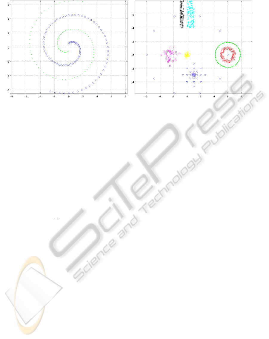
the parameters used for generating ensemble (2). Fig-
ure 1 illustrates the synthetic datasets used in the eval-
uation: (a) spiral; (b) image-c.
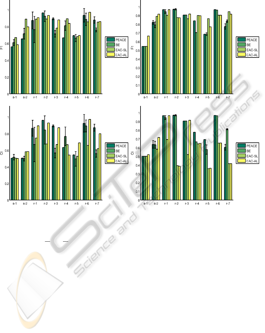
Figure 3 summarizes the average performance of
both algorithms over ensembles (1) and (2), after sev-
eral runs, accounting for possible different solutions
due to initialization, in terms of Consistency Index
(CI), and F-1 Measure.
The performance of PEACE and BE is very dif-
ferent for the synthetic and UCI datasets. On the
first, PEACE and BE have lower performance when
compared with EAC-SL and EAC-AL (both on F1
and CI); while on the later have better performance
on several examples. Comparing the performance of
both ensembles: on ensemble (1), PEACE has better
performance than other methods on 3 datasets (over
9), while on ensemble (2) it has better or equal per-
formance that the other on 6 (over 9).
Ensembles (1) were generated using a split and
merge strategy, which produces the splitting of natural
clusters into smaller clusters inducing micro-blocks
in the co-association matrix, as shown in figure 2, for
the (s-2) dataset, which has 7 natural clusters. The
results show that the proposed model is not so ad-
equate to this type of block diagonal matrix, penal-
izing PEACE. Comparing it with the BE algorithm
shows that in this complicated co-association matri-
ces, it seems that PEACE is more robust.
Ensembles (2) are generated with a combination
of several algorithms, inducing co-association matri-
ces much more blockwise, as is shown in figure 2(b).
The proposed model is much more suitable for this
type of co-association matrices. The BE algorithm
also has a better performance on this type of ensem-
bles, leading to a similar performance.
ProbabilisticEvidenceAccumulationforClusteringEnsembles
63

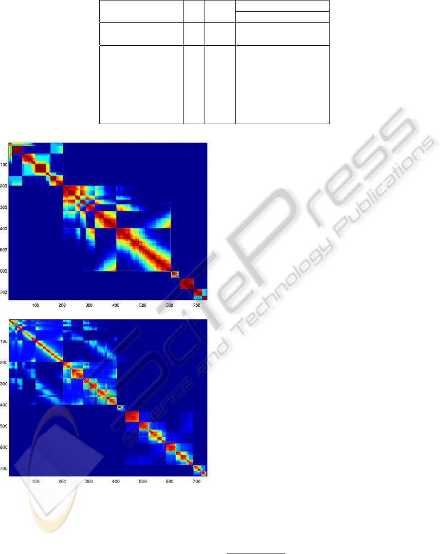
Table 1: Benchmark datasets.
Data-Sets K n
Ensemble
K
i
(s-1) spiral 2 200 2-8
(s-2) image-c 7 739 8-15,20,30
(r-1) iris 3 150 3-10,15,20
(r-2) wine 3 178 4-10,15,20
(r-3) house-votes 2 232 4-10,15,20
(r-4) ionosphere 2 351 4-10,15,20
(r-5) std-yeast-cell 5 384 5-10,15,20
(r-6) breast-cancer 2 683 3-10,15,20
(r-7) optdigits 10 1000 10, 12, 15, 20, 35, 50
(a) Ensemble 1.
(b) Ensemble 2.
Figure 2: Example of co-association Matrices obtained with
ensemble (1) and (2) - reordered using VAT (Bezdek and
Hathaway, 2002) - on the (s-2) data-set.
5.2 Text Data
We also evaluated the proposed algorithm over two
well known text-data benchmark datasets: the KDD
mininewsgroups
1
and the WebKD dataset
2
. The
mininewsgroups dataset, is composed by usenet
articles from 20 newsgroups. After removing
three newsgroups not corresponding to a clear
concept (’talk.politics.misc’, ’talk.religion.misc’,
’comp.os.ms-windows.misc’), we ended up analyz-
ing 17 newsgroups, grouped in 7 macro-categories
(’rec’,’comp’,’soc’,’sci’,’talk’,’alt’,’misc’). In this
collection there are only 100 documents on each
newsgroups, totalizing 1700 documents.
The WebKD dataset corresponds to WWW-pages
collected from computer science departments of var-
ious universities in January 1997. We concen-
trated our analysis on 4 categories ( ’project’, ’stu-
dent’, ’course’, ’faculty’). For each, we ana-
lyzed only the documents belonging to universi-
ties (’texas’,’washington’,’wisconsin’,’cornell’), to-
talizing 1041 documents.
The analysis followed the usual steps for text-
processing (Manning et al., 2008): tokenization,
stopword-removal, stemming (Porter Stemmer), fea-
ture weighting (using Tf-Idf) and feature removal.
For feature removal, we removed tokens that appeared
in less than 40 documents and words that had low
variance of occurrence, following Cui et al. (“Non-
Redundant Multi-View Clustering Via Ortogonaliza-
tion”). On the mininewsgroups dataset this feature re-
moval step, led to 500-dimension term frequency vec-
tor, while on the WebKD led to 335-dimension term
frequency vector.
We build the clustering ensembles based on the
split and merge strategy (ensemble (1)) using: K-
means with cosine similarity - ensemble 1a; and Mini-
Batch K-means algorithm (Sculley, 2010), a variant
of the classical algorithm using mini-batches (random
subset of the dataset), to compute the centroids - en-
1
http://kdd.ics.uci.edu/databases/20newsgroups/20news
groups.html
2
http://www.cs.cmu.edu/afs/cs.cmu.edu/project/theo-20
/www/data/
ICPRAM2013-InternationalConferenceonPatternRecognitionApplicationsandMethods
64

(a) F1 (Ensemble 1). (b) F1 Index (Ensemble 2).
(c) CI (Ensemble 1). (d) CI (Ensemble 2).
Figure 3: Performance Evaluation in terms of F1 and Consistency Index.
semble 1b. For the generation we assumed that each
partition had a random number of clusters, chosen in
the interval K = {
√
ns/2;
√
ns}, where ns is the num-
ber of samples.
Figure 4 illustrates an example of the obtained
coassociation matrices. To allow a better under-
standing of obtained co-association matrices, samples
are aligned according to ground truth. The block-
diagonal structure of the co-association of webKD
dataset is much more evident than on the miniNews-
groups.
In tables 2 and 3 we summarize the obtained re-
sults for the PEACE and BE algorithm, indicating
minimum, maximum, average and standard deviation
of the validation indexes. In addition, the first column
(“selected”) refers to the value of the validation index
selected according to the intrinsic optimization crite-
rion, i.e highest value of P[C|Y]. Highest values for
each data set are highlighted in bold.
From the analysis of tables 2 and 3 it is appar-
ent that the PEACE algorithm has better performance
in ensembles exhibiting higher compactness proper-
ties. However, in situations where the co-association
matrices have a less evident structure, with a lot of
noise connecting clusters, its performances tend to de-
crease.
6 CONCLUSIONS
In this paper we introduced a new probabilistic ap-
proach, based on the EAC paradigm, for consen-
sus clustering. In our model, the entries of the co-
association matrix are regarded as realizations of bi-
nomial random variables parameterized by proba-
bilistic assignments of objects to clusters, and we esti-
mate such parameters by means of a maximum likeli-
hood approach. The resulting optimization problem is
non-linear and non-convex and we addressed it using
a primal line-search algorithm. Evaluation on both
ProbabilisticEvidenceAccumulationforClusteringEnsembles
65

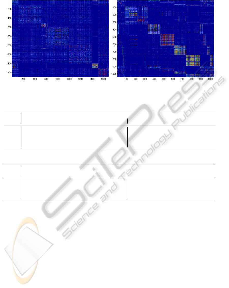
(a) miniNewsgroups. (b) webKD.
Figure 4: Examples of obtained co-associations for miniNewsgroups and webKD datasets using an ensemble of K-means
with cosine similarity.
Table 2: Consistency indices of consensus solutions for the clustering ensemble.
EnsembleData Set
PEACE BE
selected av std max min selected av std max min
E1a
miniN 0.425 0.431 0.028 0.468 0.385 0.433 0.439 0.020 0.459 0.418
webkd 0.414 0.423 0.046 0.492 0.339 0.405 0.396 0.010 0.406 0.387
E1b
miniN 0.242 0.242 0.001 0.242 0.241 0.356 0.356 0.000 0.356 0.356
webkd 0.297 0.369 0.067 0.419 0.294 0.320 0.320 0.000 0.320 0.320
Table 3: F1 of consensus solutions for the clustering ensemble.
EnsembleData Set
PEACE BE
selected av std max min selected av std max min
E1a
miniN 0.551 0.541 0.021 0.565 0.494 0.559 0.583 0.009 0.595 0.559
webkd 0.616 0.618 0.046 0.678 0.528 0.580 0.636 0.059 0.693 0.580
E1b
miniN 0.853 0.845 0.015 0.861 0.822 0.769 0.774 0.006 0.778 0.769
webkd 0.663 0.698 0.032 0.723 0.663 0.530 0.532 0.004 0.539 0.530
synthetic and real benchmarks data assessed the effec-
tiveness of our approach. As future work we want to
develop methods for exploiting the uncertainty of in-
formation given by the probabilistic assignments, as
well as exploiting the possibility of having overlap-
ping groups in the co-association matrix.
ACKNOWLEDGEMENTS
This work was partially funded by FCT
under grants SFRH/PROTEC/49512/2009,
PTDC/EIACCO/103230/2008 (EvaClue project),
and by the ADEETC from Instituto Superior de
Engenharia de Lisboa, whose support the authors
gratefully acknowledge.
REFERENCES
Ayad, H. and Kamel, M. S. (2008). Cumulative voting
consensus method for partitions with variable number
of clusters. IEEE Trans. Pattern Anal. Mach. Intell.,
30(1):160–173.
Baeza-Yates, R. A. and Ribeiro-Neto, B. (1999). Mod-
ern Information Retrieval. Addison-Wesley Longman
Publishing Co., Inc., Boston, MA, USA.
Bezdek, J. and Hathaway, R. (2002). Vat: a tool for visual
assessment of (cluster) tendency. In Neural Networks,
2002. IJCNN ’02. Proceedings of the 2002 Interna-
tional Joint Conference on, volume 3, pages 2225 –
2230.
Boyd, S. and Vandenberghe, L. (2004). Convex Optimiza-
tion. Cambridge University Press, first edition edition.
Dimitriadou, E., Weingessel, A., and Hornik, K. (2002). A
ICPRAM2013-InternationalConferenceonPatternRecognitionApplicationsandMethods
66

combination scheme for fuzzy clustering. In AFSS’02,
pages 332–338.
Fern, X. Z. and Brodley, C. E. (2004). Solving cluster en-
semble problems by bipartite graph partitioning. In
Proc ICML ’04.
Fred, A. (2001). Finding consistent clusters in data parti-
tions. In Kittler, J. and Roli, F., editors, Multiple Clas-
sifier Systems, volume 2096, pages 309–318. Springer.
Fred, A. and Jain, A. (2002). Data clustering using evidence
accumulation. In Proc. of the 16th Int’l Conference on
Pattern Recognition, pages 276–280.
Fred, A. and Jain, A. (2005). Combining multiple cluster-
ing using evidence accumulation. IEEE Trans Pattern
Analysis and Machine Intelligence, 27(6):835–850.
Ghosh, J. and Acharya, A. (2011). Cluster ensembles. Wiley
Interdisc. Rew.: Data Mining and Knowledge Discov-
ery, 1(4):305–315.
Griffiths, T. L. and Steyvers, M. (2004). Finding scientific
topics. Proc Natl Acad Sci U S A, 101 Suppl 1:5228–
5235.
Jain, A. K. and Dubes, R. (1988). Algorithms for Clustering
Data. Prentice Hall.
Kachurovskii, I. R. (1960). On monotone operators and
convex functionals. Uspekhi Mat. Nauk, 15(4):213–
215.
Lourenc¸o, A., Fred, A., and Figueiredo, M. (2011). A
generative dyadic aspect model for evidence accumu-
lation clustering. In Proc. 1st Int. Conf. Similarity-
based pattern recognition, SIMBAD’11, pages 104–
116, Berlin, Heidelberg. Springer-Verlag.
Lourenc¸o, A., Fred, A., and Jain, A. K. (2010). On the
scalability of evidence accumulation clustering. In
20th International Conference on Pattern Recognition
(ICPR), pages 782 –785, Istanbul Turkey.
Luenberger, D. G. and Ye, Y. (2008). Linear and Nonlinear
Programming. Springer, third edition edition.
Manning, C. D., Raghavan, P., and Schtze, H. (2008). In-
troduction to Information Retrieval. Cambridge Uni-
versity Press, New York, NY, USA.
Meila, M. (2003). Comparing clusterings by the variation
of information. In Springer, editor, Proc. of the Six-
teenth Annual Conf. of Computational Learning The-
ory (COLT).
Ng, A. Y., Jordan, M. I., and Weiss, Y. (2001). On spectral
clustering: Analysis and an algorithm. In NIPS, pages
849–856. MIT Press.
Rota Bul
`
o, S., Lourenc¸o, A., Fred, A., and Pelillo, M.
(2010). Pairwise probabilistic clustering using ev-
idence accumulation. In Proc. 2010 Int. Conf. on
Structural, Syntactic, and Statistical Pattern Recog-
nition, SSPR&SPR’10, pages 395–404.
Sculley, D. (2010). Web-scale k-means clustering. In
Proceedings of the 19th international conference on
World wide web, WWW ’10, pages 1177–1178, New
York, NY, USA. ACM.
Steyvers, M. and Griffiths, T. (2007). Probabilistic topic
models, chapter Latent Semantic Analysis: A Road to
Meaning. Laurence Erlbaum.
Strehl, A. and Ghosh, J. (2002). Cluster ensembles - a
knowledge reuse framework for combining multiple
partitions. J. of Machine Learning Research 3.
Topchy, A., Jain, A., and Punch, W. (2004). A mixture
model of clustering ensembles. In Proc. of the SIAM
Conf. on Data Mining.
Topchy, A., Jain, A. K., and Punch, W. (2005). Clustering
ensembles: Models of consensus and weak partitions.
IEEE Trans. Pattern Anal. Mach. Intell., 27(12):1866–
1881.
Wang, H., Shan, H., and Banerjee, A. (2009). Bayesian
cluster ensembles. In 9th SIAM Int. Conf. on Data
Mining.
Wang, P., Domeniconi, C., and Laskey, K. B. (2010). Non-
parametric bayesian clustering ensembles. In ECML
PKDD’10, pages 435–450.
ProbabilisticEvidenceAccumulationforClusteringEnsembles
67