
Evolving Classifier Ensembles using Dynamic Multi-objective
Swarm Intelligence
Jean-Franc¸ois Connolly, Eric Granger and Robert Sabourin
Laboratoire d’Imagerie, de Vision et d’Intelligence Artificielle,
´
Ecole de Technologie Sup
´
erieure, Universit
´
e du Qu
´
ebec,
1100, Rue Notre-Dame Ouest, Montreal, Canada
Keywords:
Multi-classifier Systems, Incremental Learning, Dynamic and Multi-objective Optimization, ARTMAP
Neural Networks, Video Face Recognition, Adaptive Biometrics.
Abstract:
Classification systems are often designed using a limited amount of data from complex and changing pattern
recognition environments. In applications where new reference samples become available over time, adaptive
multi-classifier systems (AMCSs) are desirable for updating class models. In this paper, an incremental learn-
ing strategy based on an aggregated dynamical niching particle swarm optimization (ADNPSO) algorithm
is proposed to efficiently evolve heterogeneous classifier ensembles in response to new reference data. This
strategy is applied to an AMCS where all parameters of a pool of fuzzy ARTMAP (FAM) neural network clas-
sifiers, each one corresponding to a PSO particle, are co-optimized such that both error rate and network size
are minimized. To sustain a high level of accuracy while minimizing the computational complexity, the AMCS
integrates information from multiple diverse classifiers, where learning is guided by the ADNPSO algorithm
that optimizes networks according both these objectives. Moreover, FAM networks are evolved to maintain
(1) genotype diversity of solutions around local optima in the optimization search space, and (2) phenotype
diversity in the objective space. Using local Pareto optimality, networks are then stored in an archive to create
a pool of base classifiers among which cost-effective ensembles are selected on the basis of accuracy, and
both genotype and phenotype diversity. Performance of the ADNPSO strategy is compared against AMCSs
where learning of FAM networks is guided through mono- and multi-objective optimization, and assessed
under different incremental learning scenarios, where new data is extracted from real-world video streams for
face recognition. Simulation results indicate that the proposed strategy provides a level of accuracy that is
comparable to that of using mono-objective optimization, yet requires only a fraction of its resources.
1 INTRODUCTION
In pattern recognition applications, matching is typi-
cally performed by comparing query samples against
class models designed with reference samples col-
lected a priori from the environment. Biometric tem-
plate matching is performed with biometric models
consisting of a set of one or more templates (reference
samples) acquired during an enrollment process, and
stored in a gallery. To improve robustness and reduce
resources, it may also consists of a statistical repre-
sentation estimated by training a classifier on refer-
ence data. Neural or statistical classifiers may implic-
itly define a model of some individual’s biometric trait
by mapping the finite set of reference samples, de-
fined in an input feature space, to an output (scores or
decision) space. Since the collection and analysis of
reference data is often expensive, these classifiers are
often designed using some prior knowledge of the un-
derlying data distributions, user-defined hyperparam-
eters, and a limited number of reference samples.
It is however possible in many biometric applica-
tions to acquire new reference samples at some point
in time after a classifier has originally been trained
and deployed for operations. Labeled and unlabeled
samples can be acquired through re-enrollment ses-
sions, post-analysis of operational data, or enrollment
of new individuals in the system, allowing for incre-
mental learning of labeled data and semi-supervised
learning of reliable unlabeled data (Jain et al., 2006;
Roli et al., 2008). Moreover, the physiology of indi-
viduals and operational condition may therefore also
change over time. In video face recognition, acquisi-
tion of faces is subject to considerable variations (e.g.,
illumination, pose, facial expression, orientation and
occlusion) due to limited control over unconstrained
operational conditions. In addition, new information,
such new individuals, may suddenly emerge, and un-
206
Connolly J., Granger E. and Sabourin R. (2013).
Evolving Classifier Ensembles using Dynamic Multi-objective Swarm Intelligence.
In Proceedings of the 2nd International Conference on Pattern Recognition Applications and Methods, pages 206-215
DOI: 10.5220/0004269302060215
Copyright
c
SciTePress

derlying data distributions may change dynamically
(e.g., aging) in the classification environment. Per-
formance may therefore decline over time as facial
models deviate from the actual data distribution. Be-
yond the need for accuracy, efficient classification
systems for various real-time applications constitutes
a challenging problem. For instance, video surveil-
lance systems use a growing numbers of IP cameras,
and must simultaneously process many video feeds,
matching facial regions to models.
Some classification systems have been proposed
for supervised incremental learning of new labeled
data, and provide the means to maintain an accu-
rate and up-to-date model of individuals (Connolly
et al., 2008). For example, the ARTMAP and Grow-
ing Self-Organizing families of neural network clas-
sifiers, have been designed with the inherent ability to
perform incremental learning. In addition, some well-
known pattern classifiers, such as the Support Vec-
tor Machine, the Multi-Layer Perceptron and Radial
Basis Function neural networks have been adapted to
perform incremental learning. However, the decline
of performance caused by knowledge (model) cor-
ruption remains a fundamental issue for monolithic
classifiers. Techniques in literature are mostly suit-
able for designing classification systems with an ad-
equate number of samples acquired from ideal and
static environments, where class distributions are bal-
anced and remain unchanged over time.
Adaptive ensemble-based techniques like some
boosting algorithms (Polikar et al., 2001), may avoid
knowledge corruption at the expense of growing sys-
tem complexity, In these cases, exploiting diversified
classifier ensembles has been shown to provide robust
and accurate systems (Kuncheva, 2004; Minku et al.,
2010; Elwell and Polikar, 2011). A key element in of
classifiers ensembles is classifier diversity measures
(Brown et al., 2005; Minku et al., 2010). Through
bias-variance error decomposition, it has been shown
empirically that considering diversity for ensemble
selection improves the generalization capabilities of
multi-classifier systems (Brown et al., 2005).
In previous work, the authors proposed an incre-
mental learning strategy driven by a dynamic parti-
cle swarm optimization (DPSO) algorithm to evolve
a heterogeneous ensemble of incremental-learning
fuzzy ARTMAP (FAM) classifiers. This strategy
was applied to an adaptive multi-classifier system
(AMCS) for video face recognition, where facial
models may be created and updated over time, as new
reference data becomes available (Connolly et al.,
2012b). In this DPSO-based strategy, each particle
corresponds to a FAM network, and the DPSO algo-
rithm co-optimizes all parameters (hyperparameters,
weights, and architecture) of a pool of base FAM clas-
sifiers such that the error rate is minimized.
While adaptation was originally performed only
according accuracy with mono-objective optimiza-
tion, the new strategy proposed in this paper is driven
by a multi-objective aggregated dynamic niching PSO
(ADNPSO) algorithm that also considers the struc-
tural complexity of FAM networks during adaptation,
allowing to design efficient heterogeneous ensem-
bles of classifiers. The ADNPSO algorithm seeks to
maintain both genotype diversity (optimization search
space) and phenotype diversity (optimization search
space) among the base classifiers during generation
and evolution of pools, and during ensemble selec-
tion, according to different criteria. The new AD-
NPSO incremental learning strategy now optimizes
all parameters of a pool of base classifiers such that
the error rate and network complexity are minimized.
An archive is proposed to store and manage non-
dominated classifiers with a Pareto-based criteria. Us-
ing local Pareto optimality, networks in the archive
are selected to design cost-effective ensembles.
The next section provides motivations for the new
incremental learning strategy based on ADNPSO.
The strategy (including ADNPSO algorithm and spe-
cialized archive) proposed evolve ensembles within
AMCSs is presented in Section 3. The data bases,
incremental learning scenarios, protocol, and perfor-
mance measures used for proof-of-concept simula-
tions are then described in Section 4, followed by
the experimental results and discussion in Section 5.
The ADNPSO learning strategy is validated on a face
recognition application in which facial models are to
be updated. Performance of AMCSs is assessed in
terms of error rate and resource requirements for in-
cremental learning of new data blocks from the real-
world video data set captured by the Institute of In-
formation Technology of the Canadian National Re-
search Council (IIT-NRC) (Gorodnichy, 2005).
2 CLASSIFICATION AND
OPTIMIZATION
2.1 Fuzzy ARTMAP Neural Network
ARTMAP refers to a family of self-organizing neu-
ral network architectures that is capable of fast, sta-
ble, on-line, unsupervised or supervised, incremen-
tal learning, classification, and prediction. A key
feature of these networks is their unique solution to
the stability-plasticity dilemma. The fuzzy ARTMAP
(FAM) integrates the unsupervised fuzzy ART neural
EvolvingClassifierEnsemblesusingDynamicMulti-objectiveSwarmIntelligence
207

Size:16 x 6 cm
Mapping
Feature space
Input feature vectors
a = (a
1
, ..., a
I
)
Decision space
Predefined
class labels
= {C
1
, ..., C
K
}
C
1
C
2
…
C
K
Search spaces
Hyperparameters
h = (h
1
, ..., h
D
)
h
2
h
1
Objective space
Objectives
o = (f
1
(h), …, f
O
(h))
Mapping
..
.
...
f
1
(h)
f
2
(h)
(a) Classification environment.
Size:16 x 6 cm
Mapping
Feature space
Input feature vectors
a = (a
1
, ..., a
I
)
Decision space
Predefined
class labels
= {C
1
, ..., C
K
}
C
1
C
2
…
C
K
Search spaces
Hyperparameters
h = (h
1
, ..., h
D
)
h
2
h
1
Objective space
Objectives
o = (f
1
(h), …, f
O
(h))
Mapping
..
.
...
f
1
(h)
f
2
(h)
Size:16 x 6 cm
Mapping
Feature space
Input feature vectors
a = (a
1
, ..., a
I
)
Decision space
Predefined
class labels
= {C
1
, ..., C
K
}
C
1
C
2
…
C
K
Search spaces
Hyperparameters
h = (h
1
, ..., h
D
)
h
2
h
1
Objective space
Objectives
o = (f
1
(h), …, f
O
(h))
Mapping
..
.
...
f
1
(h)
f
2
(h)
(b) Optimization environment.
Figure 1: Pattern classification systems may be defined according to two environments. A classification environment that
maps a R
I
input feature space to a decision space, respectively defined by feature vectors a, and a set of class labels C
k
. As the
FAM learning dynamics are govern by hyperparameter vector h, the latter interacts with an optimization environment, where
each value of h indicates a position in several search spaces, each one defined by an objective considered during the learning
process. For several objective functions (i.e., search spaces), each solution can be projected in an objective space.
network to process both analog and binary-valued in-
put patterns into the original ARTMAP architecture
(Carpenter et al., 1992). Matching query samples a
against a biometric model of individuals enrolled to
a biometric recognition system is typically the bottle-
neck, especially as the number of individuals grows.
The FAM classifier is widely used because it can per-
form supervised incremental learning of limited data
for fast and efficient matching (Granger et al., 2007).
Biometric models are learned during training by es-
timating the FAM weights, architecture and hyper-
parameters of each individual (i.e., output class) en-
rolled to the system.
Its architecture consists of three layers: (1) an in-
put layer F
1
of 2I neurons, with two neurons asso-
ciated with each input feature in R
I
, (2) a growing
competitive layer F
2
of J neurons that are each as-
sociated to an hyper-rectangle shaped prototype cate-
gory in the feature space, and (3) a map field F
ab
of K
binary output neurons, each one corresponding to an
output class. During supervised learning, FAM grows
its F
2
competitive layer to learn an arbitrary mapping
between a finite set of training patterns and their cor-
responding binary supervision patterns. It does so by
adjusting its synaptic weights to (1) create and grow
the hyper-rectangle shaped prototype categories in the
R
I
feature space to perform clustering of the available
training samples, and (2) associate those categories
(i.e., clusters) to the respective class of the training
patterns. When a query pattern is presented to the net-
work, it is propagated through the input F
1
layer and
activates a winning F
2
node. The result is a predic-
tion in the form of a binary vector of K outputs where
k = 1 corresponds to the class label of the winning F
2
node and zero elsewhere.
FAM learning dynamics are governed by four hy-
perparameters: the choice parameter α ≥ 0, the learn-
ing parameter β ∈ [0,1], the match tracking parame-
ter ε ∈ [−1, 1], and the baseline vigilance parameter
¯
ρ ∈ [0,1]. Let h = (α,β,ε,
¯
ρ) be defined as the vec-
tor of FAM hyperparameters. These are inter-related,
and each one has a distinct impact on the structure of
the hyper-rectangle shaped recognition category and
implicit decision boundaries formed during training.
Computational cost needed to operate FAM are pro-
portional its structural complexity. Given I input fea-
tures and J nodes on the growing F
2
layer, time com-
plexity to predict a class from a query sample is of
O(IJ) (Carpenter et al., 1992).
2.2 Ensembles and Dynamic MOO
Although classifier ensembles have been shown to
improve accuracy and reliability of pattern recogni-
tion systems for a wide range of applications, gen-
erating an accurate pool of classifiers and selecting
an ensemble among that pool that maximizes predic-
tion accuracy are challenging tasks. To increase di-
versity among classifiers and improve robustness of
such ensembles, swarm intelligence can be used to
guide classifiers through representation space traver-
sal (Brown et al., 2005). As illustrated in Figure 1,
swarm intelligence can be used to explore an hyper-
parameter search space defined according to a clas-
sifier. It guides different classifiers that are trained
on the same data, but using different learning dynam-
ics, to create a heterogeneous swarm of classifiers
(Valentini, 2003). The authors have shown that, since
the FAM hyperparameters govern its learning dynam-
ics, genotype diversity among solutions in the search
space indeed leads to classifier diversity in the feature
and decision spaces (Connolly et al., 2012b).
During incremental learning, adapting the FAM
classifier’s hyperparameters vector h = (α,β,ε,
¯
ρ) ac-
cording to accuracy has been shown to correspond
to a dynamic mono-objective optimization problem
(Connolly et al., 2012a). In this paper however, multi-
objective optimization (MOO) is performed in order
to maximize FAM accuracy while minimizing its net-
work computational cost, that is:
minimize f(h,t) := [ f
NS
(h,t); f
ER
(h,t)],
(1)
where f
NS
(h,t) is the network size (i.e., number of F
2
layer nodes), and f
ER
(h,t) is the generalization error
ICPRAM2013-InternationalConferenceonPatternRecognitionApplicationsandMethods
208

h
1
h
2
(a) Search space for f
1
(h).
h
1
h
2
(b) Search space for f
2
(h). (c) Objective space.
Figure 2: Position of local Pareto fronts in both search spaces an in the objective space. Obtained with a grid, true Pareto-
optimal solutions are illustrated by the dark circles and other locally Pareto-optimal solutions with light circles. While the goal
in a multi-objective optimization (MOO) is to find the true Pareto-optimal front (dark circles), another goal of the ADNPSO
algorithm is to search both search spaces to find solutions that are suitable for classifiers ensembles. For instance, if at a time
t, f
1
(h) and f
2
(h) respectively correspond to f
s
(h,t) and f
e
(h,t), these would be solutions in the red rectangle in Figures 2c
(with low generalization error and for a wide range of FAM network F
2
sizes).
rate of the FAM network for a given hyperparame-
ter vector h and after learning data set D
t
at a dis-
creet time t (Connolly et al., 2012a). Although it was
not verified, it is assumed in this paper that training
FAM with different values of h leads to different num-
ber of FAM F
2
nodes and that the objective function
f
NS
(h,t) also corresponds to a dynamic optimization
problem.
As a MOO problem, the first goal of the optimiza-
tion module is to find the Pareto-optimal front of non-
dominated solutions. Given the set of objectives o to
minimize, a vector h
d
in the hyperparameter space is
said to dominate another vector h if:
∀o ∈ o : f
o
(h
d
) ≤ f
o
(h), and
∃o ∈ o : f
o
(h
d
) < f
o
(h).
(2)
The Pareto-optimal set, defining a Pareto front, is the
set of non-dominated solutions.
When adapting classifiers through incremental
learning, another goal of the optimization algorithm
is to seek hyperparameter values that will give a di-
versified pool of FAM networks among which accu-
rate ensembles may be selected. As illustrated in Fig-
ure 2 with a simple MOO problem, the optimization
process should provide accurate solutions with differ-
ent network structural complexities. This results in
ensembles with good generalization capabilities, but
with a possibility of having a moderate overall com-
putational complexity.
In this particular case, an optimization algorithm
should tackle a dynamic optimization problem by
considering several objectives, and yield classifiers
that corresponds to vectors h that are not necessarily
Pareto-optimal (see Figure 2). Classic DPSO algo-
rithms as well as MOO algorithms, such as NSGA,
MOEA, MOSPO, etc. are not well suited for such
problems. The only approach in literature that is
aimed at generating and evolving a population of
FAM networks that are diverse in term of struc-
tural complexity, yet contained non-dominated alter-
natives, is presented in (Li et al., 2010). In this
case, a memetic archive was instead used to prune F
2
layer nodes and categorize FAM networks into sub-
populations that evolved independently according to
some genetic algorithm. With this method, FAM net-
works must be pruned to maintain phenotype diver-
sity and can only be applied when they are accessible,
which is not the case in the present paper.
3 EVOLUTION OF ENSEMBLES
This paper seeks to address challenges related to the
design of robust AMCSs, where class models are
designed and updated over time as new reference
data becomes available. In this section, a new AD-
NPSO incremental learning strategy – integrating an
aggregated dynamical niching PSO (ADNPSO) al-
gorithm and a specialized archive – is described to
evolve heterogeneous classifier ensembles in response
to new data. Each particle in the optimization envi-
ronment corresponds to a FAM network in the clas-
sification environment, and the ADNPSO learning
strategy evolves a swarm of classifiers such that both
FAM error rate and network size are minimized.
3.1 Adaptive Multi-classifier Systems
Figure 3 depicts the evolution of an adaptive multi-
classifier system (AMCS) for incremental learning of
new data. It is composed of (1) a long term mem-
ory (LTM) that stores and manages incoming data for
validation, (2) a population of base classifiers, each
one suitable for supervised incremental learning, (3)
EvolvingClassifierEnsemblesusingDynamicMulti-objectiveSwarmIntelligence
209

hyp
t-1
Size: 16.5 cm x 4.3 cm
Hyper-
parameters
Fitness
ADNPSO
module
LTM
t
D
t
hyp
t
Adaptive multiclassifier system
Selection
and fusion
+
Archive
(pool of
classifiers)
Swarm of
incremental
classifiers
Figure 3: Evolution over time of the adaptive multi-classifier system (AMCS) in a generic incremental learning scenario,
where new blocks of data are used to update a swarm of classifiers. Let D
1
, D
2
, ... be blocks of training data that become
available at different instants in time t = 1, 2, .... The AMCS starts with an initial hypothesis hyp
0
from prior knowledge of
the classification environment. Given a new data blocks D
t
, each hypothesis hyp
t−1
is updated to hyp
t
by the AMCS.
a dynamic population-based optimization module that
tunes the user-defined hyperparameters of each clas-
sifier, (4) a specialized archive to keep a pool of clas-
sifiers for ensemble selection, and (5) an ensemble se-
lection and fusion module.
When a new block of learning data D
t
becomes
available to the system at a discrete time t, it is em-
ployed to update the long term memory (LTM), and
evolve the swarm of incremental classifiers. The LTM
stores data samples from each individual class for val-
idation during incremental learning and fitness esti-
mation of particles on the objective function (Con-
nolly et al., 2012a). Each particle in the search spaces
are associated to a FAM network, and the ADNPSO
module, through a learning strategy, co-jointly de-
termines the classifiers hyperparameters, architecture,
and parameters such that FAM networks error rate
and size are minimized. A specialized archive stores
a pool of classifiers, corresponding to locally non-
dominated solutions (of different structural complex-
ity) found during the optimization process. Once the
optimization process is complete, the selection and
fusion module produces an heterogeneous ensemble
that is combined with a simple majority vote.
3.2 Aggregated Dynamical Niching PSO
Particle swarm optimization (PSO) is a swarm in-
telligence stochastic optimization technique that is
inspired by social behavior of bird flocking or fish
schooling. With PSO, each particle corresponds to a
single solution in the optimization environment, and
the population of particles is called a swarm. In a
mono-objective problem and at a discreet iteration
τ, particles move through the hyperparameter search
space and change their positions h(τ) under the guid-
ance of different sources of influence. Unlike evolu-
tionary algorithms (such as genetic algorithms), each
particle always keeps in memory its best position and
the best position of its surrounding. PSO algorithms
use this information and move the swarm according
to a social influence (i.e., their neighborhood previ-
ous search experience) and a cognitive influence (i.e.,
their own previous search experience).
To tackle ensemble creation, ADNPSO uses the
same approach as mono-objective optimization algo-
rithms and defines influences in the search spaces,
with the objective functions. As Figure 2 previously
showed with a simple problem, the rational behind
this approach is that when several local optima are
present in different search spaces, non-dominated so-
lutions tend to be located in regions between local op-
tima of the different objective. Each particle will then
move according to a cognitive and social influence for
error rate (ER) and network size (NS) objectives (see
Figure 4). Formally this is defined by:
h(τ + 1) = h(τ) + w
0
(h(τ) − h(τ − 1))
+ r
1
w
1
(h
soc., ER
− h(τ)) + r
2
w
2
(h
cog., ER
− h(τ))
+ r
3
w
3
(h
soc., NS
− h(τ)) + r
4
w
4
(h
cog., NS
− h(τ)),
(3)
During optimization, each particle (1) begins at its
current location, (2) continues moving in the same di-
rection it was going according to an inertia weight
w
0
, and (3) is attracted by each source of influence
according to a weight w
θ
adjusted by random num-
bers r
θ
. By adjusting the weights w
θ
, the swarm may
be biased according to one objectives or even divided
in three sub-populations : (1) one that specializes in
accuracy (w
1
and w
2
> w
3
and w
4
), (2) one that spe-
cializes in complexity (w
1
and w
2
< w
3
and w
4
), and
(3) a generalist subpopulation that put both objectives
on equal footing (w
1
= w
2
= w
3
= w
4
).
Social influences of both objectives are managed
by creating subswarms by adapting the DNPSO lo-
cal neighborhood topology (Nickabadi et al., 2008) to
multiple objectives. While DNPSO dynamically cre-
ates subswarms around the current position of local
best particles that are particles with a personal best
ICPRAM2013-InternationalConferenceonPatternRecognitionApplicationsandMethods
210
h
1
h
2
1
Personal best
positions
1
2
Subswarm
2
2
(a) Search space for f
1
(h).
h
1
h
2
2
Local best
positions
2
1
1
1
Personal best
positions
Subswarm
2
Subswarm
(b) Search space for f
2
(h).
h
1
h
2
1
2
1
2
2
2
2
2
1
1
1
(c) Particle movements.
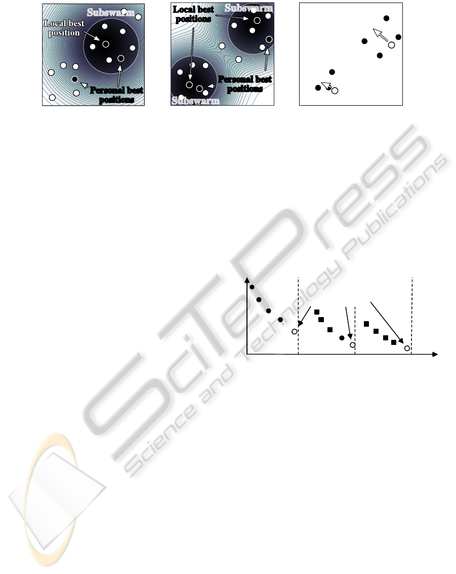
Figure 4: Examples of influences in the search spaces and resulting movements. Given the same objective functions used in
Figure 2, two particles among a swarm (white circles), and their social and cognitive influences (black circles), let subswarms
set to have a maximal size of 5 particles. While both particles 1 and 2 are going to have cognitive influences in both search
spaces, particle 1 is not part of any subswarm for f
1
(h). Unlike particle 2, it has no social influence for this objective and
ADNPSO sets w
1
= 0 when computing its movement with Equation 3.
position that has the best fitness in their neighbor-
hood, the ADNPSO rather use the memory of these
(local best) particles. Social influences are then per-
sonal best position of local best particles computed
independently for both objectives. As shown in Fig-
ure 4, by limiting the size of each subswarm, particles
can be excluded of these subswarms for none, one, or
both objectives. For the objective for which it is ex-
cluded, it is said to be free and its social influence is
removed by setting the weights w
1
= 0 and/or w
3
= 0
when computing Equation 3. This way, poor compro-
mises can be avoided and conflicting influences can
then be managed simply by limiting the maximal size
of each subswarm.
Although the DNPSO local neighborhood topol-
ogy insures in many ways particle diversity in the
search space, it is also adapted to also maintain cog-
nitive (i.e., personal best) diversity among particles
within each subswarm. The ADNPSO algorithm de-
fines a distance ∆ around local best positions of each
objectives. Every time a particle moves with the dis-
tance ∆ from the detected local optima of one objec-
tive, “loses its memory” for that objective by erasing
its personal best value. It then moves only according
the other objectives b settings the proper weights to 0.
3.3 Archive and Ensemble Selection
Since a limited amount of reference data is used to de-
sign the AMCS, both objectives are discrete function,
and the accuracy (error rate) is prone to over fitting. In
this context, a specialized archive is used to (1) insure
phenotype diversity in the objective space according
to FAM network size, and (2) as framework for en-
semble selection.
As Figure 5 shows, it categorizes FAM networks
associated with each solution found in the search
space according to their network size and stores them
to create a pool of classifiers among which ensembles
can be selected. Although, for a MOO formulation,
this imply keeping dominated solutions in the objec-
tive space, using a specialized archive ensures storing
classifiers with a wide phenotype diversity for FAM
network F
2
layer size.
FAM network size (number of F
2
nodes)
Error rate (%)
Size = 7 x 3
Phenotype
local best
Figure 5: Specialized archive in the objective space. The
FAM network size objective is segmented in different do-
mains, where both Pareto-optimal (circles) and locally
Pareto-optimal (squares) solutions are stored. The local best
are defined as the most accurate network of each domain.
While a genotype local best topology in the hy-
perparameter space is used to define neighborhoods
and zones of influence for the different particles, the
same principle is applied in the objective space for
ensemble selection. The most accurate FAM of each
network size domain are considered as phenotype lo-
cal best solutions. Classifiers are selected to create an
initial ensemble that is completed with a second se-
lection phase that uses a greedy search process (intro-
duced in (Connolly et al., 2012b)) to increase classi-
fier diversity by maximizing their genotype diversity.
3.4 ADNPSO Learning Strategy
An ADNPSO incremental learning strategy (Algo-
rithm 1) is proposed to evolve FAM networks accord-
ing multiple objectives and accumulate a pool of FAM
EvolvingClassifierEnsemblesusingDynamicMulti-objectiveSwarmIntelligence
211

networks in the archive presented in Section 3.3. Dur-
ing incremental learning of a data block D
t
, FAM
hyperparameters, parameters and architecture are co-
jointly optimized such that the generalization error
rate and network size are minimized. Based on the hy-
pothesis that maintaining diversity among particles in
the optimization environment implicitly generates di-
versity among classifiers in the classification environ-
ment (Connolly et al., 2012b), properties of the AD-
NPSO algorithm is used to evolve a diversified het-
erogeneous ensembles of FAM networks over time.
At a time t, and for each particle n, the current par-
ticle position is noted h
n
, along with its personal best
values on each objective function o, h
∗
n,o
. The values
estimated on the objective functions and the best po-
sition of each particle are respectively noted f
o
(h
n
,t)
and f
o
(h
∗
n,o
,t). For O objectives, and the ADNPSO
algorithm presented in Section 3.2 that uses N parti-
cles, a total of (O + 2)N FAM networks are required.
For each particle n, the AMCS stores:
1. O networks FAM
n,o
associated with h
∗
n,o
(particle
n personal best position on each objective func-
tion o),
2. the network FAM
start
n
associated to the current po-
sition of the each particle n after convergence of
the optimization process at time t − 1, and
3. the network FAM
est
n
obtained after learning D
t
with current position of particle n (noted h
n
).
While FAM
start
n
represents the state of the particle be-
fore learning D
t
, FAM
est
n
is the state of the same par-
ticle after having explored a position in the search
space, and it is used for fitness estimation.
During the initialization process (line 1), the
swarm and all FAM networks are initialized. Par-
ticle positions are randomly initialized within their
allowed range. When a new D
t
becomes available,
the optimization process begins. Networks associated
with the best position of each particle (FAM
n,o
) are
incrementally updated using D
t
, along with their fit-
ness f
o
(h
∗
n,o
,t) (lines 3–5). Network in the archive
and their fitness are also updated in the same man-
ner (lines 6–13). Since accuracy corresponds to dy-
namic optimization problem, Algorithm 1 verifies if
solutions still respect the non-dominant criteria of the
specialized archive. Then, the specialized archive is
filled accordingly using networks FAM
n,o
.
Optimization continues were it previously ended
until the ADNPSO algorithm converges (lines 14–
27). During this process, the ADNPSO algorithm ex-
plores the search spaces (line 15). A copy of FAM
start
n
redefines the state of FAM
est
prior learning at a time
t, trains the latter using h
n
, and estimates its fitness
(lines 17–19). For each objective o, the best position
(h
∗
n,o
) and its corresponding fitness ( f
o
(h
∗
n,o
,t)) and
network (FAM
n,o
) are updated if necessary (lines 20–
26). If f
o
(h
n
,t) and f
o
(h
∗
n,o
,t) are equal, the network
that requires the least resources (F
2
nodes) is used.
Each time fitness is estimated at a particle current po-
sition, FAM
est
is categorize according its network size
and added to the archive if it is non-dominated in its
F
2
size domain (lines 23–26). Finally, the iteration
counter is incremented (line 27). Once optimization
converges, networks corresponding to the last posi-
tion evaluated of every particle (FAM
est
n
) are stored in
FAM
start
n
(lines 28–29). These networks will define the
swarm’s state prior learning data block D
t+1
.
4 EXPERIMENTAL
METHODOLOGY
Proof-of-concept simulations focus on classification
of facial regions captured in a video face recogni-
tion applications. Since matching is perform with an
AMCS based on adaptive FAM ensembles, systems
responses for each successive query sample is a bi-
nary code (equals to “1” for the predicted class, and
“0”s for the others).
The data base was collected by the Institute for In-
formation Technology of the Canadian National Re-
search Council (IIT-NRC) (Gorodnichy, 2005). It
is composed of 22 video sequences captured from
eleven individuals positioned in front of a computer.
For each individual, two color video sequences of
about fifteen seconds are captured at a rate of 20
frames per seconds with an Intel web cam of a 160 ×
120 resolution that was mounted on a computer mon-
itor. Of the two video sequences, one is dedicated to
training and the other to testing. They are taken under
approximately the same illumination conditions, the
same setup, almost the same background, and each
face occupies between 1/4 to 1/8 of the image. This
data base contains a variety of challenging operational
conditions such as motion blur, out of focus factor, fa-
cial orientation, facial expression, occlusion, and low
resolution. The number of ROIs detected varies from
class to class, ranging from 40 to 190 for one video
sequences.
Segmentation is performed using the well known
Viola-Jones algorithm included in the OpenCV
C/C++ computer vision library. In both cases, re-
gions of interest (ROIs) produced are converted in
gray scale and normalized to 24 × 24 images where
the eyes are aligned horizontally, with a distance of
12 pixels between them. Principal Component Analy-
sis is then performed to reduce the number of features.
The 64 features with the greatest eigenvalues are ex-
tracted and vectorized into a = {a
1
,a
2
,...,a
64
}, where
each feature a
i
∈ [0,1] are normalized using the min-
ICPRAM2013-InternationalConferenceonPatternRecognitionApplicationsandMethods
212

max technique. Learning is done with ROIs extracted
from the first series of video sequences (1527 ROIs
for all individuals) while testing is done with ROIs
extracted from the second series of video sequences
Algorithm 1: ADNPSO incremental learning strategy.
Inputs: An AMCS and new data sets D
t
for learning.
Outputs: An ensemble of FAM networks.
Initialization:
1: • Set the swarm and archive parameters,
• Initialize all (O + 2)N networks,
• Set PSO iteration counter at τ = 0, and
• Randomly initialize particles positions and velocities.
Upon reception of a new data block D
t
, the following
incremental process is initiated:
Update FAM
n,o
associated to the personal best posi-
tions:
2: for each particle n, where 1 ≤ n ≤ N do
3: for each objectives o, where 1 ≤ o ≤ O do
4: Train FAM
n,o
with validation.
5: Estimate f
o
(h
∗
n,o
,t).
Update the archive:
6: Update the accuracy of each solution in the archive.
7: Remove locally dominated solutions form the archive.
8: for each particle n, where 1 ≤ n ≤ N do
9: for each objectives o, where 1 ≤ o ≤ O do
10: Categorize FAM
n,o
.
11: if FAM
n,o
is a non-dominated solution for its net-
work size domain then
12: Add the solution to the archive.
13: Remove solutions from the archive that are lo-
cally dominated by FAM
n,o
.
Optimization process:
14: while stopping conditions are not reached do
15: Update particle positions according to the ADNPSO
algorithm (Equation 3).
Estimate fitness and update personal best positions:
16: for each particle n, where 1 ≤ n ≤ N do
17: FAM
est
n
← FAM
start
n
18: Train FAM
est
n
with validation.
19: Estimate f
o
(h
n
,t) of each objective.
20: for each objective o, where 1 ≤ o ≤ O do
21: if f
o
(h
n
,t) < f
o
(h
∗
n,o
,t) then
22: { h
∗
n,o
, FAM
n,o
, f
o
(h
∗
n,o
,t) } ← { h
n
,
FAM
est
n
, f
o
(h
n
,t) }.
Update the archive:
23: Categorize FAM
est
n
24: if FAM
est
n
is locally non-dominated then
25: Add the solution to the archive
26: Remove solutions from the archive that are lo-
cally dominated by FAM
est
n
.
27: Increment iterations: τ = τ + 1.
Define initial conditions for D
t+1
:
28: for each particle n, where 1 ≤ n ≤ N do
29: FAM
start
n
← FAM
est
n
.
(1585 ROIs for all individuals).
Prior to simulations, each video data set is divided
into blocks of data D
t
, where 1 ≤ t ≤ T , to emulate
the availability of T successive blocks of training data
to the AMCS. Supervised incremental learning is per-
formed according to an update learning scenario. All
classes are initially learned with the first block D
1
; at
a given time, face images of an individual becomes
available and then learned by the AMCS to refined
its internal models. In order to assess performance
in cases where classes are initially ill defined, D
1
is
composed of 10% of the data for each class, and each
subsequent block D
t
, where 2 ≤ t ≤ K + 1, is com-
posed of the remaining 90% of one specific class.
The performance of the proposed ADNPSO learn-
ing strategy is evaluated using different optimization
algorithms and different ensemble selection meth-
ods during supervised incremental learning of data
blocks D
t
. The parameters used are shown in Table
1. Weight values {w
1
,w
2
} were defined as proposed
in (Kennedy, 2007), and to detect a maximal num-
ber of local optima, no constraints were considered
regarding the number of subswarm. Since Euclidean
distances between particles are measured during opti-
mization, the swarm evolves in a normalized R
4
space
to avoid any bias due to the domain of each hyperpa-
rameter. Before being applied to FAM, particle po-
sitions are de-normalized to fit the hyperparameters
domain. For each new blocks of data D
t
, the opti-
mization is set to either stop after 10 iterations with-
out improving the performance of either generaliza-
tion error rate of network size, or after maximum 100
iterations. Learning is performed over 10 trials using
ten-fold cross-validation. Incoming data is managed
with the LTM as specified in (Connolly et al., 2012a).
Each trial is repeated with five different class presen-
tation orders, for a total of fifty replications.
Table 1: ADNPSO parameters.
Parameter Value
Swarm’s size N 60
Weights {w
1
,w
2
} {0.73,2.9}
Maximal size of each subswarm 4
Neighborhood size 5
Minimal distance between two local best 0.1
Minimal velocities of free particles 0.0001
Performance is evaluated for (1) an AMCS that
uses the incremental learning strategy as described in
Section 3: ADNPSO ← the networks in the special-
ized archive corresponding to the phenotype local best
plus a greedy search that maximizes genotype diver-
sity (Connolly et al., 2012b). This system is compared
to AMCSs using the ADNPSO learning strategy used
EvolvingClassifierEnsemblesusingDynamicMulti-objectiveSwarmIntelligence
213

Table 2: Error rates and complexity indicators after incre-
mental learning of data base. Complexity is evaluated in
terms of ensemble size, average network F
2
layer size, and
total F
2
layer size for the entire ensemble. Average values
are presented with a 90% confidence interval.
Method ADNPSO DNPSO MOPSO
Error rate (%) 22.4±0.6 22.7±0.7 26.9±0.7
Ensemble size 5.5 ± 0.4 12.4 ± 0.8 7.9 ± 0.6
Av. nb. of F
2
nodes 170±9 108±5 52±3
Tot. nb. of F
2
nodes 900±100 1300±100 420±50
with different optimization algorithms and ensemble
selection techniques: (2) DNPSO ← the ensemble of
FAM networks associated to the local best positions
found with the mono-objective DNPSO (Nickabadi
et al., 2008) plus a greedy search within the swarm to
maximize genotype diversity (Connolly et al., 2012b),
and (3) MOPSO ← the entire archive obtained with
the ADNPSO incremental learning strategy employed
with the multi-objective PSO algorithm that uses
the notion of dominance to guide particles toward
the Pareto optimal front (Coello et al., 2004). The
MOPSO algorithm was used with the same applica-
ble parameters than with the proposed ADNPSO, and
with a grid size of 10 (for further details, see (Coello
et al., 2004)).
The average performance of AMCSs is assessed
in terms of generalization error and structural com-
plexity. The error rate is the ratio of incorrect pre-
dictions over all test set predictions, where each face
images is tested independently. Structural complexity
is measure in terms of the number of nodes on the F
2
layer of all FAM networks in the ensemble.
5 RESULTS AND DISCUSSION
As depicted in Table 2, results indicate that using the
proposed ADNPSO provides a level of accuracy that
is comparable to that of using mono-objective opti-
mization (DNPSO) but with a fraction of the compu-
tational cost. While the average network size of en-
sembles obtained with ADNPSO is the highest among
all methods, the average ensemble size gives a to-
tal number of F
2
nodes that is lower than mono-
objective optimization. On the other hand, while
multi-objective PSO (MOPSO) yields the lightest en-
sembles, the error rate is on average 4% higher than
that obtained with the other methods.
Table 3 shows performance with the average parti-
cle position and standard deviation after learning the
whole data base. When the proposed ADNPSO di-
rects subswarms of particles according information in
the search spaces, rather than in the objective space,
the swarm is able to remain dispersed in the objec-
Table 3: Average value and standard deviation of the
swarm’s current position after learning the entire IIT-NRC
data base. Results are shown for the error rate and number
of F
2
layer nodes, with a 90% confidence interval.
Method ADNPSO DNPSO MOPSO
Average value
Error rate(%) 35±2 19±1 45±2
Nb. of F
2
nodes 100±3 195±5 20±1
Standard deviation
Error rate(%) 22±1 17±1 32±1
Nb. of F
2
nodes 110±5 90±4 10±1
tive space according both error rate and network size.
The specialized archive insures that the most accurate
solutions are stored for different network sizes.
On the other hand, with mono-objective optimiza-
tion according only to accuracy (DNPSO), FAM net-
works tend to continuously grow their F2 layer to
maintain or increase accuracy. The swarm then tends
to have a higher level of accuracy with less variations,
but with a much higher computational cost. Some par-
ticles are however still able to perform well with low
structural complexities, explaining the relatively high
dispersion for the number of F
2
nodes.
If influences are define in the objective space with
the MOPSO algorithm, Table 3 shows that using clas-
sifiers such as FAM introduces a bias in the swarm’s
movements toward structural complexity. Theoret-
ically, the MOO algorithms considers both objec-
tives equally. However, given the nature of the prob-
lem (evolving FAM networks over time), a conven-
tional MOO approach will find non-dominated so-
lutions with fewer F
2
nodes more easily than non-
dominated solutions with lower error rate. Particles
in the different search spaces are then directed such
as mostly minimizing FAM network size, thus limit-
ing the search capabilities for accurate solutions.
6 CONCLUSIONS
This paper presents an incremental learning strategy
based on ADNPSO that allows to evolve ensembles
of heterogeneous classifiers in response to new ref-
erence data. This strategy is applied to an AMCS
where all parameters of a swarm of FAM neural net-
work classifiers (i.e., a swarm of classifiers), each one
corresponding to a particle, are co-optimized such
that both error rate and network size are minimized.
Multi-objective minimization is performed such that
genotype diversity of solutions around local optima
in the optimization search space, and phenotype di-
versity in the objective space are maintained. By us-
ing the specialized archive, local Pareto-optimal solu-
tions detected by the ADNPSO algorithm can also be
ICPRAM2013-InternationalConferenceonPatternRecognitionApplicationsandMethods
214

stored and combined with a greedy search algorithm
to create ensembles based on accuracy, phenotype and
genotype diversity.
Overall results indicates that using information in
the search space of each objective (local optima po-
sitions and values), rather than in the objective space,
permits creating pools of classifiers that are more ac-
curate and with lower computational cost. For in-
cremental learning scenarios with real-world video
streams, ADNPSO provides accuracy comparable to
that of using mono-objective optimization, yet re-
quires a fraction of its computational cost. Since
the proposed AMCS is designed with samples col-
lected from changing classification environments, fu-
ture work will focus on measures to detect various
types of changes in the feature space (see Figure 1).
This information could then be used to trigger an up-
date of the pool and archive only when new data in-
corporated relevant information.
ACKNOWLEDGEMENTS
This research was supported by the Natural Sciences
and Engineering Research Council of Canada.
REFERENCES
Brown, G., Wyatt, J., Harris, R., and Yao, X. (2005). Di-
versity creation methods: a survey and categorization.
Information Fusion, 29(6):5–20.
Carpenter, G. A., Grossberg, S., Markuzon, N., Reynolds,
J. H., and Rosen, D. B. (1992). Fuzzy artmap: A neu-
ral network architecture for incremental supervised
learning of analog multidimensional maps. IEEE
Transactions on Systems, Man, and Cybernetics C,
3(5):698–713.
Coello, C., Pulido, G., and Lechuga, M. (2004). Han-
dling multiple objectives with particle swarm opti-
mization. IEEE Transactions on Evolutionary Com-
putation, 8(3):256–279.
Connolly, J.-F., Granger, E., and Sabourin, R. (2008). Su-
pervised incremental learning with the fuzzy artmap
neural network. In Proceedings of the Artificial Neu-
ral Networks in Pattern Recognition, pages 66–77,
Paris, France.
Connolly, J.-F., Granger, E., and Sabourin, R. (2012a).
An adaptive classification system for video-based face
recognition. Information Sciences, 192(1):50–70.
Swarm Intelligence and Its Applications.
Connolly, J.-F., Granger, E., and Sabourin, R. (2012b).
Evolution of heterogeneous ensembles through dy-
namic particle swarm optimization for video-based
face recognition. Pattern Recognition, 45(7):2460–
2477.
Elwell, R. and Polikar, R. (2011). Incremental learning
of concept drift in nonstationary environments. IEEE
Transactions on Neural Networks, 22(10):1517–1531.
Gorodnichy, D. O. (2005). Video-based framework for face
recognition in video. In Second Workshop on Face
Processing in Video in Proceedings of the Conference
on Computer and Robot Vision, pages 325–344, Vic-
toria, Canada.
Granger, E., Henniges, P., Oliveira, L. S., and Sabourin, R.
(2007). Supervised learning of fuzzy artmap neural
networks through particle swarm optimization. Jour-
nal of Pattern Recognition Research, 2(1):27–60.
Jain, A. K., Ross, A., and Pankanti, S. (2006). Biometrics:
A tool for information security. IEEE Transactions on
Information Forensics and Security, 1(2):125–143.
Kennedy, J. (2007). Some issues and practices for particle
swarms. In Proceedings of the IEEE International on
Swarm Intelligence, pages 162–169, Honolulu, USA.
Kuncheva, L. I. (2004). Classifier ensembles for chang-
ing environments. In Proceedings of the International
Workshop on Multiple Classifier Systems, pages 1–15,
Cagliari, Italy.
Li, R., Mersch, T. R., Wen, O. X., Kaylani, A., and Anag-
nostopoulos, G. C. (2010). Multi-objective memetic
evolution of art-based classifiers. In Proceedings
of the IEEE Congress on Evolutionary Computation,
pages 1–8, Barcelona, Spain.
Minku, L. L., White, A. P., and Yao, X. (2010). The impact
of diversity on online ensemble learning in the pres-
ence of concept drift. IEEE Transactions on Knowl-
edge and Data Engineering, 22(5):730–742.
Nickabadi, A., Ebadzadeh, M. M., and Safabakhsh, R.
(2008). DNPSO: A dynamic niching particle swarm
optimizer for multi-modal optimization. In Proceed-
ings of the IEEE Congress on Evolutionary Computa-
tion, pages 26–32, Hong Kong, China.
Polikar, R., Udpa, L., Udpa, S. S., and Honavar, V. (2001).
Learn++ : An incremental learning algorithm for su-
pervised neural networks. IEEE Transactions on Sys-
tems, Man, and Cybernetics C, 31(4):497–508.
Roli, F., Didaci, L., and Marcialis, G. (2008). Adaptive bio-
metric systems that can improve with use. In Ratha,
N. K. and Govindaraju, V., editors, Advances in Bio-
metrics, pages 447–471. Springer London.
Valentini, G. (2003). Ensemble methods based on bias-
variance analysis. PhD thesis, University of Genova,
Genova, Switzerland.
EvolvingClassifierEnsemblesusingDynamicMulti-objectiveSwarmIntelligence
215
