
Smart Classifier Selection for Activity Recognition on Wearable Devices
Negar Ghourchian and Doina Precup
McGill University, Montreal, Canada
Keywords:
Activity Recognition, Sensor Selection, Active Learning.
Abstract:
Activity recognition is a key component of human-machine interaction applications. Information obtained
from sensors in smart wearable devices is especially valuable, because these devices have become ubiquitous,
and they record large amounts of data. Machine learning algorithms can then be used to process this data.
However, wearable devices impose restrictions in terms of computation and energy resources, which need
to be taken into account by a learning algorithm. We propose to use a real-time learning approach, which
interactively determines the most effective set of modalities (or features) for classification, given the task at
hand. Our algorithm optimizes sensor selection, in order to consume less power, while still maintaining good
accuracy in classifying sequences of activities. Performance on a large, noisy dataset including four different
sensing modalities shows that this is a promising approach.
1 INTRODUCTION
Recognizing everyday activities is an active area of
research in machine learning and context-aware com-
puting. Classical work for estimating user behavior in
activity recognition is based on high dimensional and
densely sampled video streams (Clarkson and Pent-
land, 1999). However, these approaches are intrusive
and power-inefficient when monitoring in real-world
conditions over a long period of time. For such situa-
tions, real-time sensory information obtained through
smart wearable devices is preferable, because such
devices have become ubiquitous. Many of these de-
vices come equipped with sensors such as GPS, ac-
celerometer, digital compass, gyroscope, barometer,
WiFi and infrared, which can query the local envi-
ronment and yield information about the user’s activ-
ities. For example, mobile phone sensing can be used
in personal health-care, safety and fitness, by moni-
toring and analysing the daily physical activities and
body movement of a user.
Most existing work includes as many sensory
modalities as possible to produce a large, complex
feature vector, including low-level features like fre-
quency content, or higher-level measures like number
of objects detected by the proximity sensor (Choud-
hury et al., 2008; Mannini and Sabatini, 2010; Sub-
ramanya and Raj, 2006). Then, feature selection is
needed to determine which of these features are use-
ful for classification. The techniques of sensor select-
ion can be broadly classified into two main cate-
gories (Zhang and Ji, 2005). The greedy search-based
approach regards sensor selection as a heuristic search
problem (Kalandros et al., 1999). The decision-
theoretic approach regards sensor selection as a de-
cision making problem (Castanon, 1997). However,
both approaches suffer from combinatorial explosion.
Moreover, if a real-time activity detection task runs on
a smart phone, all the sensors are typically always on,
and a lot of additional computing power is required
by the heavy-duty feature extraction and feature se-
lection tools. While these approaches work well, at
the end all algorithms select a single feature vector
(including features from all sensors) to classify every
different type of activity, which often requires all the
sensors to be engaged all the time. This is subopti-
mal from the point of view of energy and computation
load on the device.
We propose a real-time activity recognition algo-
rithm which actively selects a smaller subset of sen-
sors that are the most informative, yet cost-effective,
for each time frame. We use a greedy process to dis-
cover sets of sensor modalities that most influence
each specific activity. These subsets of sensors are
then used to build different models for the activities.
We use these models to develop an algorithm that de-
cides on-line which model is suitable for recognizing
the activity in each given time frame. Our algorithm
has the flavor of active learning (Settles, 2010), but
instead of asking for labels on new data points, we
581
Ghourchian N. and Precup D. (2013).
Smart Classifier Selection for Activity Recognition on Wearable Devices.
In Proceedings of the 2nd International Conference on Pattern Recognition Applications and Methods, pages 581-585
DOI: 10.5220/0004269805810585
Copyright
c
SciTePress

start the recognition task with a small set of sensors
and then interactively send queries for more features,
as needed. In this way, we can afford to run the activ-
ity recognition engine on a low-powered device with-
out sacrificing the accuracy. We present empirical re-
sults on real data, which illustrate the utility of this
approach.
2 METHODOLOGY AND DATA
The data set used for the feature selection experi-
ment was collected by Dieter Fox (Subramanya and
Raj, 2006), using the Intel Mobile Sensing Platform
(MSP (Choudhury et al., 2008) that contains several
sensors, including 3-axis accelerometer, 3-axis gyro-
scope, visible light photo transistor, barometer, and
humidity and ambient light sensors. Six participants
wore the MSP units on a belt at the side of their
hip and were asked to perform six different activities
(walking, lingering, running, climbing upstairs, walk-
ing downstairs and riding a vehicle) over a period of
three weeks. Ground truth was acquired through ob-
servers who marked the start and end points of the
activities. The working data set was 50 hours of la-
belled data (excluding the beginning of each record-
ing which was labelled as unannotated) and also
some long sequences (over 1 minute) labelled as un-
known. There were also some short unlabelled seg-
ments, which we smoothed out using a moving aver-
age filter. We computed the magnitude of the accel-
eration
p
x
2
+ y
2
+ z
2
based on components sampled
at 512 Hz. We also used the gyroscope (sampled at
64Hz), barometric pressure (sampled at 7.1Hz) and
visible light (sampled at 3Hz). These four measures
were all up-sampled to 512Hz in order to obtain time
series of equal length. To prevent overfitting to char-
acteristics of the locations, we did not include the hu-
midity and temperature sensors, as they could poten-
tially mislead the classifier to report a false correla-
tion between location and activities. For example, if a
lot of walking data were collected under hot sun, the
classifier would see temperature as a relevant feature
to walking.
For the classification task, we used random for-
est (Breiman, 2001), a state-of-the-art ensemble clas-
sifier which also provides a certainty measure in the
classification. The random forest algorithm builds
many classification trees, where each tree votes for
a class and the forest chooses the majority label. As-
sume we have N instances in the training set and there
are M tests (based on the features) for each instance.
In order to grow a tree, N instances are sampled at
random with replacement and form the training set.
At each node, m M tests are randomly chosen and
the best one of these is determined. Each tree grows
until all leaves are pure, i.e. no pruning is performed.
A subset of the training set (normally about one-third
of the N instances) are left out to be used as a valida-
tion set, to get a running estimate of the classification
error as trees are added to the forest. The error on this
out-of-bag (OOB) data gives an unbiased error esti-
mate. This classifier is very efficient computationally
during both training and predicting, while maintain-
ing good accuracy.
We also need an probabilistic certainty measure,
which should reflect how confident the classification
is. We will use this quantity to manage the sensor
selection procedure. When using random forests, for
any given sample in the validation set, the classifier
not only predicts a label, but also reports what pro-
portion of the votes given by all trees matches the pre-
dicted label. We used this ratio as a certainty measure.
3 INITIAL EXPERIMENTS WITH
SENSOR SELECTION
Table 1: Individual classifiers. The bold line in each section
denotes the classifier with the highest accuracy.
No. Feature Set Accuracy
1 {Acc, Bar, Gyro, VisLight} 86.16
2 {Acc, Bar, Gyro} 75.16
3 {Acc, Bar, VisLight} 86.50
4 {Acc, Gyro, VisLight} 84.33
5 {Bar, Gyro, VisLight} 78.33
6 {Bar, Gyro} 54.00
7 {Acc, Gyro} 69.50
8 {Acc, Bar} 74.83
9 {Acc, VisLight} 77.66
10 {Bar, VisLight} 74.00
11 {Gyro, VisLight} 74.00
12 {Acc} 48.16
First, we wanted to verify the effect of differ-
ent subsets of sensors on the accuracy of recogniz-
ing the six different activities. We began by examin-
ing all possible combinations of sensors on the entire
data set. We treated each time sample as an instance
and used raw sensor data as features for classifica-
tion task. We performed cross-validation over users
(leaving in turn each user’s dataset aside as the test
set and combining and randomizing all other datasets
to use as training set) The accuracy of the classifiers
for all 12 possible combination sets of four sensors
1
1
Single features except the accelerometer are excluded
from the results due to poor performance.
ICPRAM2013-InternationalConferenceonPatternRecognitionApplicationsandMethods
582

is given in Table 1. From now on, instead of full sen-
sor names, we use abbreviations Acc, Bar, Gyro and
VisLight for accelerometer, barometric pressure, gy-
roscope and ambient visible light, respectively.
The overall results are competitive with prior ac-
tivity recognition results that used complex feature
sets, even though we used the raw sensory values.
It is also clear that not all sensors are contributing
equally to the performance. For example, compar-
ing results from classifiers No.1 and No.3 in Table 1
clearly shows that data from the gyroscope did not
provide useful information about this set of activities.
Moreover, this sensor seems to lead to a similar or
less improvement than the barometer sensor. So we
decided to prune the gyroscope.
The contribution of each sensor varies among dif-
ferent activities. For example, accelerometer data is
key in discriminating physical activities such as run-
ning and walking. However, the classifier using only
accelerometer data (No.12) performs poorly while
recognizing some activities like riding a vehicle or
while distinguishing activities with similar dynamics
(e.g. upstairs vs. downstairs). However, this classifier
is the cheapest one in terms of energy consumption
and it is reliable enough to be used as a default clas-
sifier for our active learner. There is smaller subset of
sensors which models well this set of activities. Clas-
sifiers No.3 and No.9 achieved 86.5% and 77.66% ac-
curacy rate, respectively, whereas the classifier No.1
(using all sensors) only obtained 86.16%. Hence, we
identified subsets that can be used instead of the full
set of sensors.
4 PROPOSED APPROACH FOR
SENSOR SELECTION
In this section we introduce a real-time algorithm
that optimally selects the best classifier for each time
frame. The main idea is to start the activity recog-
nition task by acquiring data just from the single
most informative sensor and building a cheap classi-
fier. The certainty measure provided by this classifier
is then used to identify points in time when uncer-
tainty is high, so using more sensors could be benefi-
cial. Other classifiers can then be invoked. Figure 1
presents an overview of the information flow.
The algorithm begins by training a set of classi-
fiers, each using a feature set selected in advance,
based on application-specific criteria. The experiment
in previous section is an example of how the best fea-
ture sets can be chosen, though one would not need
to be so exhaustive. In general, the set of classifiers
should contain at least one cheap classifier that can
Figure 1: Overview of the algorithm.
run all the time, and an expensive classifier with very
good accuracy. Also, if there is a large number of sen-
sor modalities, it is useful to have some classifiers that
use different types of resources, not only for energy
consumption, but also to ensure that the application
is robust with respect to sensor failure, or unusually
noisy readings.
When the training phase is over, the algorithm will
have to process new time series. It starts by sliding
a fixed-width window (of length w), with 10% over-
lap, over the data, in order to obtain data intervals.
We would like to keep the length of these intervals
as small as possible, in order to avoid mixtures of
activities, but large enough to capture the essence of
the activity. Each interval is initially labelled by the
cheapest classifier. We compute the running average
of the certainty measure over each frame, to indicate
if the classifier is confident enough about the labelling
decision or not. If the measure drops below a given
threshold, the algorithm will query other sensors, and
upgrade the classifier to a more complex one, which
works with the new information.
The algorithm will switch back to a cheaper clas-
sifier as soon as its certainty measure rises above the
threshold. To do this, the algorithm simultaneously
computes and compares the confidence level of both
classifiers at each time frame, and switches back when
the threshold is exceeded again. Ideally, we want the
algorithm to have smooth transitions between classi-
fiers, so we also use a control parameter, which allows
the algorithm to switch from one model to another
only after δ frames.
SmartClassifierSelectionforActivityRecognitiononWearableDevices
583
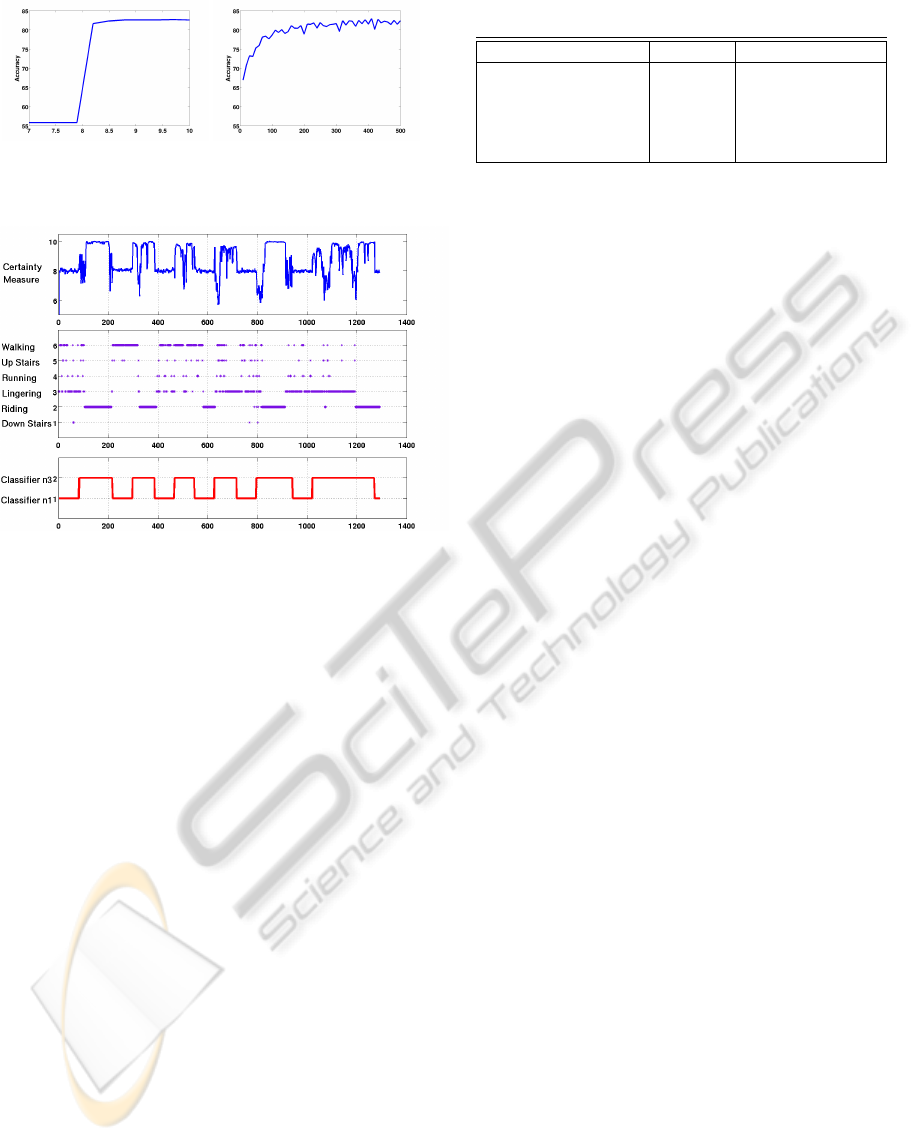
(a) (b)
Figure 2: Influence of θ (left) and δ (right) on performance.
Figure 3: Algorithm performance on a segment of data. The
top and middle figures show the the certainty measure of
the classifier in use and the corresponding true activities at
each time frame. The bottom figure shows the algorithm’s
decision of the best classifier to use.
5 RESULTS AND DISCUSSION
We evaluated the proposed algorithm on the data
set and selected subsets from the experiment in
Sec. 3. The number of classifiers used is N = 3,
where the classifiers to be tried are n
1
= {Acc},
n
2
= {Acc, VisLight} and n
3
= {Acc, Bar, VisLight}.
Hence, the algorithm will first use only the accelerom-
eter data for classification, then incorporate visible
light, and in the worst case, barometric pressure as
well. In both training and testing we used 10 trees in
the forest
There are two parameters that were chosen empir-
ically, and which influence the results:
• δ, the number of frames before switching to an-
other classifier is allowed
• θ, the threshold for the certainty measure, which
may depend on the overall accuracy rate
Figure 2 shows how δ and θ affect the overall accu-
racy of the system. One can see that performance is
stable for a fairly large range of these parameters.
In practice, we found that switching between two
classifiers, instead of three, yields better accuracy and
Table 2: Comparison of recognition accuracy.
Algorithm Accuracy Proportion of time
Classifier n
1
48.16 100%
Classifier n
2
77.66 100%
Classifier n
3
86.50 100%
Active alg.(n
1
, n
2
, n
3
) 71.78 9%,32%,59%
Active alg.(n
1
, n
3
) 80.14 35%,65%
smoother transitions. This happens because the al-
gorithm does not stay with n
2
for long and tends to
switch between n
1
and n
3
. Figure 3 shows a run of
the algorithm on a segment of data from one specific
user, using classifiers trained on the other users’ data.
Table 2 shows the classification results of the pro-
posed algorithm and the baselines from the first ex-
periment, as well as the proportion of the time the
algorithm used each classifier. The overall accuracy
of the active algorithm (combination of 2 classifiers)
is just 6% lower than the best baseline(n
3
) while con-
suming 35% less energy. This is significant savings
for a low-powered device.
6 FINAL REMARKS
We presented an approach that can be used to select
among classifiers with different features (and power
consumption) in activity recognition tasks. the active-
learning-style idea is to use a certainty measure in the
result of the classification to decide if a more “ex-
pert” classifier should provide labels. However, no
input from a user is required, as the algorithm is fully
automatic. The empirical results show that our ap-
proach can successfully switch between complex and
simple classifiers, on-line and in real time, yielding
power savings without significant loss in accuracy. In
future work, we aim to further explore the empirical
and theoretical properties of this algorithm. We are
also exploring the use of reinforcement learning, in-
stead of active learning, for this problem. Reinforce-
ment learning has the advantage of being able to in-
corporate and balance in a quantitative fashion power
savings and accuracy changes.
ACKNOWLEDGEMENTS
This research was sponsored in part by FQRNT and
NSERC.
ICPRAM2013-InternationalConferenceonPatternRecognitionApplicationsandMethods
584

REFERENCES
Breiman, L. (2001). Random forests. Machine Learning,
45(1):5–32.
Castanon, D. A. (1997). Approximate dynamic program-
ming for sensor management. In IEEE CDC, pages
1202–1207.
Choudhury, T., Consolvo, S., Harrison, B., Hightower, J.,
LaMarca, A., LeGrand, L., Rahimi, A., Rea, A., Bor-
dello, G., Hemingway, B., Klasnja, P., Koscher, K.,
Landay, J., Lester, J., Wyatt, D., and Haehnel, D.
(2008). The mobile sensing platform: An embed-
ded activity recognition system. Pervasive Comput-
ing, 7(2):32–41.
Clarkson, B. and Pentland, A. (1999). Unsupervised clus-
tering of ambulatory audio and video. In ICASSP,
pages 3037–3040.
Kalandros, M., Pao, L. Y., and Chi Ho, Y. (1999). Random-
ization and super-heuristics in choosing sensor sets
for target tracking applications. In IEEE CDC, pages
1803–1808.
Mannini, A. and Sabatini, A. M. (2010). Machine learning
methods for classifying human physical activity from
on-body accelerometers. Sensors, 10(2):1154–1175.
Settles, B. (2010). Active learning literature survey. Tech-
nical Report 1648, University of Wisconsin-Madison.
Subramanya, A. and Raj, A. (2006). Recognizing activities
and spatial context using wearable sensors. In UAI.
Zhang, Y. and Ji, Q. (2005). Sensor selection for active
information fusion. In AAAI, pages 1229–1234.
SmartClassifierSelectionforActivityRecognitiononWearableDevices
585
