Bayesian Estimation of Camera Characteristics including Spectral
Sensitivities from a Color Chart Image without Manual Parameter
Tuning
Yusuke Murayama, Pengchang Zhang and Ari Ide-Ektessabi
Graduate School of Engineering, Kyoto University, Kyoto, Japan
Keywords:
Camera Characterization, Bayesian Estimation, Marginalized Likelihood, Spectral Sensitivity, Linearization.
Abstract:
We proposed a new practical method for identifying characteristics of a color digital camera: spectral sensi-
tivity function, linearization function and noise variance of each color channel. The only input is an image
of a color chart acquired by the objective camera with a spectral-content-known illuminant, and the camera
characteristics are obtained automatically. The proposed method was developed in the Bayesian statistical
framework in order to improve upon previous methods, namely, to eliminate trial-and-error parameter tuning
and to identify linearization function as well as spectral sensitivities. The polyline linearization function and
the noise variance of a color channel were considered as hyperparameters, and estimated by the marginalized
likelihood criterion. Such hyperparameters associated with the smoothness of the sensitivity curves were also
estimated similarly. Then the spectral sensitivity of a color channel was obtained as maximum a posteriori
solution. In experiments using synthetic data, the proposed method was found to be widely adaptable to the
forms of sensitivity curves and the levels of sensor noise.
1 INTRODUCTION
Spectral sensitivities of color channels are one of the
most important characteristics of a color imaging de-
vices such as an RGB camera because this character-
istic determines the color separation and the colori-
metric behavior of the device. Spectral sensitivities
are needed to be known for various advanced appli-
cations of an imaging device as well as for evalua-
tion of color reproduction and for color calibration
(Sharma and Trussell, 1997; Urban and Grigat, 2009),
such as spectral reflectance estimation (Shen and Xin,
2006), image deblurring and noise reduction (Urban
et al., 2008), and image superresolution (Murayama
and Ide-Ektessabi, 2012).
Unfortunately, manufacturers usually don’t pro-
vide detailed characteristics of their imaging devices
including spectral sensitivities. Though we could
measure spectral sensitivities by using a monochrom-
eter and a spectroradiometer (Vora et al., 1997), it
takes much time and effort for the adjustment and
measurement process. The quite high cost of these
equipments is also an obstacle.
As a solution, researchers have been developing
indirect methods for recovering spectral sensitivities
from camera responses for a color chart. This ap-
proach has the advantage of practicality because we
only have to prepare a color chart with known spec-
tral reflectance, and illuminate it uniformly by using
a light source with known spectral power distribu-
tion, and then acquire an image of the color chart.
The spectral sensitivity of a color channel is obtained
by solving a regression problem between the sensor
responses and the spectrum reflected from the color
chart patches. The early issue in spectral sensitivity
recovery is how to stabilize the regression problem
because it is a typical ill-conditioned problem, which
means a small amount of noise included in the data is
dramatically amplified to the regression solution.
Sharma and Trussell (1996) proposed to introduce
constraints of spectral sensitivity: non-negativity,
smoothness, modality, etc. They calculated a solution
which satisfies the all constraints and doesn’t make
the radial errors of sensor responses over a certain
value by applying the computationaltechnique of pro-
jections onto convex sets. Finlayson et al. (1998) also
used similar constraints, but represented spectral sen-
sitivity through a small number of Fourier basis func-
tions, instead of adopting the constraint of smooth-
ness. They formulate the spectral sensitivity recovery
as a constrained minimization problem which can be
solved by the quadratic programming. Due to these
15
Murayama Y., Zhang P. and Ide-Ektessabi A..
Bayesian Estimation of Camera Characteristics including Spectral Sensitivities from a Color Chart Image without Manual Parameter Tuning.
DOI: 10.5220/0004271600150022
In Proceedings of the International Conference on Computer Vision Theory and Applications (VISAPP-2013), pages 15-22
ISBN: 978-989-8565-47-1
Copyright
c
 2013 SCITEPRESS (Science and Technology Publications, Lda.)

devices, the recovery of spectral sensitivities was en-
abled in the presence of a relatively high amount of
sensor noise.
As an additional issue, Barnard and Funt (2002)
pointed out that a nonlinear characteristic of sensor
response declined the accuracy of spectral sensitivity
recovery, and performed a linearization at the same
time of recovering the spectral sensitivity. The lin-
earization of sensor response is necessary in all ap-
plications mentioned above. Though the linearization
function can be identified from images of same scene
captured with different exposures(Grossberg and Na-
yar, 2006), Barnard and Funt’s approach is reasonable
because of its possibility of improving accuracy in
spectral sensitivity recovery as well of its efficiency.
Beside the linearization, they proposed to add a reg-
ularization term to the cost function of the regres-
sion problem instead of using Fourier basis functions.
Regularization is a well-known technique for improv-
ing ill-conditioned regression. A regularization term
is generally represented by a norm of a variant to
be recovered, and they adopted the second derivative
norm to smooth the recovered sensitivity.
However, there remains a practical issue of se-
lecting tuning parameters. For example, the smooth-
ness of a recovered spectral sensitivity depends on the
threshold value in Sharma and Trussell’s method, the
total number of Fourier basis functions in Finlayson
et al.’s method, and the regularization coefficient in
Barnard and Funt’s method. These are typical tun-
ing parameters, which need to be selected through
trial-and-error process. Besides in Barnard and Funt’s
method, the linearization function was given paramet-
rically based on the empirical knowledge of their ob-
jective camera, and some of the parameters were ad-
justed with trial and error. Though Carvalho et al.
(2004) proposed a scheme to determine all tuning pa-
rameters in Finlayson et al.’s method objectively by
adopting an extended criterion of cross validation,
they didn’t deal with the linearization of sensor re-
sponses.
This study aims to develop a method for identi-
fying spectral sensitivity functions and linearization
functions without manual parameter tuning and with
simple implementation. We formalized the problem
of spectral sensitivity recovery in the Bayesian sta-
tistical framework. A smooth regularization and a
nonnegative constraint were adopted, and they were
introduced to our Bayesian model as a prior distribu-
tion. A polyline function was used for linearization,
which achieves a high degree of freedom in calibra-
tion regardless of camera choices. The noise vari-
ance as well as the spectral sensitivity and the lin-
earization function of a color channel can be identi-
fied from a color chart image owing to the modeling
in the Bayesian framework. In this study we show the
Bayesian formalization, and the implementation of its
solution. We also show experiments using synthetic
data.
2 PROPOSED METHOD FOR
IDENTIFYING CAMERA
CHARACTERISTICS
2.1 Outline of Bayesian Estimation
Let θ
k
(λ) be the spectral sensitivity of a camera, and
y
(i)
k
its sensor response for the i-th color patch of
a color chart (i = 1, ...,N), where k and λ denote
color channel (k =R,G,B) and wavelength respec-
tively. The parameter to be obtained is the sensitiv-
ity θ
k
(λ) and is estimated by a conditional probabil-
ity p(θ
k
(λ)|y
k
) called the posterior, where we denote
a set of sensor responses of k-channel by the vector
y
k
= [y
(1)
k
·· · y
(N)
k
]
T
.
The posterior is derived from the likelihood
p(y
k
|θ
k
(λ)) and the prior p(θ
k
(λ)) by applying the
Bayesian theorem on conditional probability:
p(θ
k
(λ)|y
k
) =
p(y
k
|θ
k
(λ))p(θ
k
(λ))
R
p(y
k
|θ
k
(λ))p(θ
k
(λ))dθ
k
(λ)
. (1)
The likelihood represents an input-output model of
the camera, and the prior represents the prior knowl-
edge about spectral sensitivity curves which can be
utilized to exclude the possibility of inappropriate so-
lutions, and to make the sensitivity recovery stable.
The spectral sensitivity of the color channel is ob-
tained as the maximum a posteriori (MAP) estimator,
which is the maximum point of the posterior and a
common estimator.
In the Bayesian framework, parameters included
in the likelihood or the prior can be determined in a
data-driven manner. Such parameters are called hy-
perparameters, and we introduce the camera charac-
teristics except spectral sensitivity as hyperparame-
ters of the Bayesian model. An effective criterion
for hyperparameter estimation is the log-marginalized
likelihood h defined by
h = ln
Z
p(y
k
|θ
k
(λ))p(θ
k
(λ))dθ
k
(λ), (2)
where the marginalization by unknown sensitivity
θ
k
(λ) helps avoid over-fit estimation (Bishop, 2006).
The maximization of h can be solved by repeated cal-
culation of the expectation-maximization (EM) algo-
rithm (Bishop, 2006). In E-step, the posterior is cal-
VISAPP2013-InternationalConferenceonComputerVisionTheoryandApplications
16

culated using provisional parameters and then the ex-
pectation value of the log-likelihood with respect to
the provisional posterior is calculated. In M-step, hy-
perparameters are renewed such that they maximize
the expectation value obtained in E-step. These two
steps are repeated until convergence.
The proposed method is executed separately in
each color channel. Hereafter we omit the color chan-
nel index k for easier readability.
2.2 Nonlinear Camera Model and
Likelihood
RGB cameras are modeled by the following equation
at each pixel (Sharma and Trussell, 1996; Barnard and
Funt, 2002):
y =
Z
θ(λ)x(λ)dλ + ε, (3)
where x(λ) is the input spectra, y and θ(λ) are the sen-
sor response and the spectral sensitivity of a certain
color channel, and ε is the sensor noise. The input
spectra x(λ) can be obtained as the product of spec-
tral power distribution of the illuminant and spectral
reflectance of the object at the pixel.
In the case that the sensor has a nonlinear char-
acteristic, Eq.(3) should be applied after converting
the real sensor response z to the linearized response
y. Let f be a monotonically increasing function for
linearizing z with respect to input light intensity. In
this study, we normalize z and y to range [0,1] and
consider a polyline function at regular intervals as the
linearization function f:
y =f(z;{α})
=α
i

z−
i−1
M−1

+ α
i+1

i
M−1
− z

for
i−1
M−1
≤ z ≤
i
M−1
,
(4)
where {α} = {α
1
,. .. ,α
M
} are the polyline points,
and they are constrained by 0 ≤ α
1
≤ ··· ≤ α
M
= 1.
Functions of wavelength such as θ(λ) and x(λ) are
vectorized by wavelength-sampling for the sake of
computing. We denote them by vectors θ and x whose
dimensions are the wavelength samplings Λ respec-
tively.
The likelihood is derived by assuming a Gaussian
noise and applying the camera model to each color
patches of an acquired color chart image as follows:
p(z|θ) =
N
∏
i=1
N (y|θ
T
x
(i)
,σ
2
)
= N (y|Xθ,σ
2
I
N
),
(5)
where X = [x
(1)
·· · x
(N)
]
T
, z = [z
(1)
·· · z
(N)
]
T
and the
superscripts of x and z indicate the color patch num-
ber. N (t|µ,Σ) denotes the univariate or multivariate
Gaussian distribution of t whose mean or mean vector
is µ and whose variance or variance matrix is Σ, and
I
N
denotes the identity matrix of size N.
2.3 Prior Knowledge about Spectral
Sensitivity
We introduce a prior reflecting the non-negativity and
the smoothness of spectral sensitivity curves as fol-
lows:
p(θ) =
(
aN (θ|0,ω
2
(D
T
r
D
r
)
−1
) θ ≥ 0
0 otherwise
(6)
where ω is a scale parameter, D
r
is a (Λ + r)-by-Λ
matrix representing the r-th degree differential
matrix with zero padding, and a is the normal-
ization constant. The i-th column vector of D
r
is
[0,...,0
| {z }
i−1
,(−1)
r
r
C
r
,(−1)
r−1
r
C
r−1
,. .. ,
r
C
0
| {z }
r+1
,0,. .. ,0
| {z }
Λ−i
]
T
,
for example,
D
2
=







1
−2 1
1 −2
.
.
.
1
.
.
.
1
.
.
.
−2
1







,
D
3
=









−1
3 −1
−3 3
.
.
.
1 −3
.
.
.
−1
1
.
.
.
3
.
.
.
−3
1









.
(7)
The first r rows and the last r rows of D
r
are added
by zero padding to reflect the boundedness, namely
that spectral sensitivity closes to zero at both ends
of wavelength range. r is related to the smoothness.
Figure 1 shows spectral sensitivities sampled from
the prior p(θ). It can be seen how smooth sensi-
tivities are supposed by adopting this prior and that
the smoothness increases as increasing r. In Fig-
ure 1 ω fixed to 1 but affects the scale of the ver-
tical axis. This prior is equivalent to introducing
a regularization term of
1
ω
2
kD
r
θk
2
in the previous
non-Bayesian methods. The 2nd differential matrix
without zero padding was used in both Sharma and
Trussell’s method and Barnard and Funt’smethod, but
we add zero padding and determine the degree r in
data-driven manner. In our method, the optimum de-
gree of r is estimated as well as ω. a doesn’t need to
be calculated.
BayesianEstimationofCameraCharacteristicsincludingSpectralSensitivitiesfromaColorChartImagewithoutManual
ParameterTuning
17

(i)
400 450 500 550 600 650 700
0
5
10
15
20
25
30
35
Wavelength [nm ]
Sensitivity [a.u.]
400 450 500 550 600 650 700
0
20
40
60
80
100
120
Wavelength [nm ]
Sensitivity [a.u.]
(ii)
Figure 1: Spectral sensitivities sampled from the prior with
different r-values where ω was fixed to be 1.
2.4 Implementation
The posterior is derived from Eqs.(1),(5) and (6) and
standard matrix operations as follows:
p(θ|z) =
(
bN (θ|µ,Σ) θ ≥ 0
0 otherwise
(8)
with
Σ =

1
σ
2
X
T
X +
1
ω
2
D
T
r
D
r

−1
(9)
µ =
1
σ
2
ΣX
T
y, (10)
where b is the normalization constant. This poste-
rior is represented as a truncated multivariate Gaus-
sian distribution as well as the prior we introduced,
but we employ quadratic approximation in order to
avoid high-dimensional numerical integration for ob-
taining b. The approximated posterior ˜p(θ|z) is rep-
resented as a complete multivariate Gaussian distribu-
tion as follows:
˜p(θ|z) = N (θ|µ
MAP
,Σ) (11)
with
µ
MAP
= arg max
θ
p(θ|y)
= arg min
θ≥0
(θ− µ)
T
Σ
−1
(θ− µ)
= arg min
θ≥0
h
θ
T
Σ
−1
θ−
2
σ
2
y
T
Xθ
i
.
(12)
The EM algorithm is applied to find hyperpa-
rameters {{α}, σ, ω} such that they maximize the
marginalized log-likelihood when r is fixed. In our
implementation, initially, {α} was set so as to repre-
sent a simple linear function, and both σ and ω were
set to 1. {{α}
new
,σ
new
,ω
new
} are set to the initial val-
ues, and the EM algorithm is implemented as follows:
E-step

{α}
old
,σ
old
,ω
old

← {{α}
new
,σ
new
,ω
new
},
y ← f(z,{α}
old
),
Σ ←

1
(σ
old
)
2
X
T
X +
1
(ω
old
)
2
D
T
r
D
r

−1
,
µ ←
1
(σ
old
)
2
ΣX
T
y, and
µ
MAP
← arg min
θ≥0
h
θ
T
Σ
−1
θ−
2
σ
2
y
T
Xθ
i
.
M-step
{α}
new
= arg min
0≤α
(1)
≤···≤α
(M)
=1
k f(z;{α}
old
) − Xµk
2
,
y ← f(z,{α}
new
),
σ
new
←
1
N
p
ky− Xµk
2
+ tr(ΣXX
T
), and
ω
new
←
1
Λ
p
kD
r
µk
2
+ tr(ΣD
T
r
D
r
).
These two steps are repeated, where perhaps several
tens of times are enough to convergence. Both mini-
mizations to update µ
MAP
in E-step and {α} in M-step
can be solved by the quadratic programming (QP)
algorithm with low computational cost. The QP al-
gorithm was used in Finlayson et al’s method and
Barnard and Funt’s method. The detailed implemen-
tation of the minimization in M-step, which is poly-
line fitting by the QP method, is described in Aronov
et al, 2004 . The spectral sensitivity, polyline points
for linearization and noise variance are obtained by
the latest values of µ
MAP
, {α} and σ
2
respectively for
a certain r. r is chosen as a natural number, such that
the marginalized log-likelihood h is minimized. h is
derived by applying the same approximation as the
posterior as follows:
h =
1
2
lndet(2πΣ) −
1
2
lndet(2πσ
2
I
N
)
−
1
2
lndet(2πω
2
(D
T
r
D
r
)
−1
)
−
1
2
σ
2
kyk
2
−
1
2
µ
T
MAP
Σ
−1
µ
MAP
.
(13)
3 RESULTS ON SYNTHETIC
DATA
We have tested the proposed method on spectral sen-
VISAPP2013-InternationalConferenceonComputerVisionTheoryandApplications
18

Table 1: Comparison of the errors in recovering spectral sensitivities in the case of linear sensor responses. These results
correspond to those in Figure 1.
RMSE of spectral sensitivity (×10
−5
)
Method Sony DXC-930 camera Kodak DCS-460 camera
R ch. G ch. B ch. R ch. G ch. B ch.
Poposed method 8.00 2.24 4.19 5.89 2.00 2.24
Method A 5.15 3.03 12.51 3.72 2.38 3.97
Method B 8.54 1.98 2.05 4.67 2.03 2.91
sitivities of two commercial cameras: Sony DCX-930
and Kodak DCS-200. The former camera has sensi-
tivity curves like Gaussian functions while the latter
camera’s sensitivities have more complicated forms.
The former was used in Barnard and Funt (2004), and
the latter was in Finlayson et al. (1998) and Car-
valho et al. (2004). The spectral sensitivities of the
two cameras were obtained from a spectral sensitivity
database (Zhao, ). In this experiment, 288 input spec-
trum were prepared from spectral reflectance of IT8
target, which is a common color chart, and spectral
power distribution of D65 standard illuminant. Spec-
tral reflectance of each color patch was measured by
ourselves using X-rite SP64 spectrocolorimeter. Both
the sensitivities and the spectrum were sampled from
400 nm to 700 nm at 10 nm wavelength intervals. The
first experiment (Sec. 3.1) compared our method with
two previous methods with only respect to the accu-
racy of spectral sensitivity recovery. It was performed
supposing linear sensor responses because the previ-
ous methods don’t have the ability of automatic lin-
earization. The second experiment (Sec. 3.2) dealt
with linearization of sensor responses under several
noise levels, and evaluated the accuracy of the cam-
era characteristics identified by the proposed method.
The true values of spectral sensitivities were normal-
ized such that sensor responses become 1 for 100-
percent diffuse reflection, namely that perfect white
is represented by y
R
= y
G
= y
B
= 1.
3.1 Linear Sensor Response
We supposed 1% additive noise and set the standard
deviation of sensor noise σ to 0.01 in each color chan-
nel. The sensor responses of the two cameras were
produced according to Eqs. (3) and (4) where the lin-
earization function f was set to the identity function.
Three methods were applied to recover the sensitiv-
ities: Our proposed Bayesian method, Finlayson et
al.’s method using Fourier basis functions with modal-
ity constraints (Method A), and Barnard and Funt’s
method using smooth regularizations and range con-
straints (Method B). Method A adopts the squared ab-
solute residue of sensor response as the cost function
in the regression while Method B adopts the squared
residue divided by sensor response. Nonnegativecon-
straints were adopted in all of the three methods. In
this experiment, tuning parameters of Method A and
Method B were chosen correctly or optimally. The
details are as follows: both the peak wavelength of a
sensitivity in Method A and the wavelength range in
which a sensitivity is zero in Method B were given
based on the true spectral sensitivity, and both the to-
tal number of Fourier basis in Method A and the reg-
ularization parameter in Method B were selected such
that the root-mean-square error (RMSE) of the recov-
ered sensitivity is the minimum. Figure 1 and Table 1
show the results and the RMSEs in spectral sensitiv-
ity recovery with respect to methods. Results of the
proposed method were resemble to those of Method
B, and they achieved high accuracy regardless of the
forms and the ranges of spectral sensitivities. Method
A provided better recovery in the red channel of Ko-
dak DCS-200 camera, whose sensitivity curvewas the
most complex in this experiment, but not good recov-
ery in the blue channel of Sony DCX-930 camera.
Our method selected hyperparameters automatically
but nevertheless it achieved as high accuracy on the
whole as the other two methods.
3.2 Nonlinear Sensor Response
A gamma characteristic was supposed as the nonlin-
earity of sensor responses, which is defined by:
z = y
1/γ
or y = z
γ
. (14)
γ was set to 2.2, which approximates the nonlin-
ear characteristic of familiar sRGB-based cameras.
We tested our method in three levels of noise: σ =
0.002, 0.01, 0.05, namely 0.2%, 1% and 5% additive
noise. Table 2 shows the RMSEs of the spectral sen-
sitivities recovered by the proposed Bayesian method.
Though the recovery accuracy declined as increasing
noise level, relatively-high accuracy was achieved in
spite of the nonlinearity of sensor responses. Figure
2 shows the identified linearization functions. There
occurred small gaps only in the dark range of the red
channel and the green channel of the Kodak camera.
Table 3 shows the errors of the identified standard de-
viation of the sensor noises. In all cases the noise
BayesianEstimationofCameraCharacteristicsincludingSpectralSensitivitiesfromaColorChartImagewithoutManual
ParameterTuning
19

400 450 500 550 600 650 700
0.0
0.5
1.0
1.5
Wavelength [nm ]
Sensitivity [a.u.]
10
- 3
Sony DXC−930 camera
400 450 500 550 600 650 700
0.0
0.2
0.4
0.6
0.8
1.0
1.2
1.4
Wavelength [nm ]
Sensitivity [a.u.]
10
- 3
Kodak DCS−460 camera
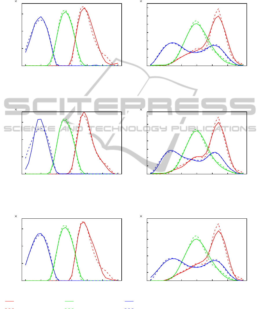
(ii) Method A: Minimizing the sum of the squared absolute errors of sensor responses
with the constraints of nonnegativity and modality and Fourier basis
R channel (recovered)
R channel (true)
G channel (recovered)
G channel (true)
B channel (recovered)
B channel (true)
400 450 500 550 600 650 700
0.0
0.5
1.0
1.5
Wavelength [nm ]
Sensitivity [a.u.]
10
- 3
Sony DXC−930 camera
400 450 500 550 600 650 700
0.0
0.2
0.4
0.6
0.8
1.0
1.2
1.4
Wavelength [nm ]
Sensitivity [a.u.]
10
- 3
Kodak DCS−460 camera
(i) Proposed Bayesian method
0.0
0.5
1.0
1.5
Sensitivity [a.u.]
10
- 3
400 450 500 550 600 650 700
Wavelength [nm ]
Sony DXC−930 camera
400 450 500 550 600 650 700
0.0
0.2
0.4
0.6
0.8
1.0
1.2
1.4
Wavelength [nm ]
Sensitivity [a.u.]
10
- 3
Kodak DCS−460 camera
(iii) Method B: Minimizing the sum of the squared relative errors of sensor responses
with the constraints of nonnegativity and range and with smooth regularizaton
Figure 2: Results of the recovered spectral sensitivities in the case of linear sensor responses. The proposed method and two
previous methods were compared using synthetic data on two commercial cameras. 1% noise (σ = 0.01) was added to the
sensor response data.
VISAPP2013-InternationalConferenceonComputerVisionTheoryandApplications
20

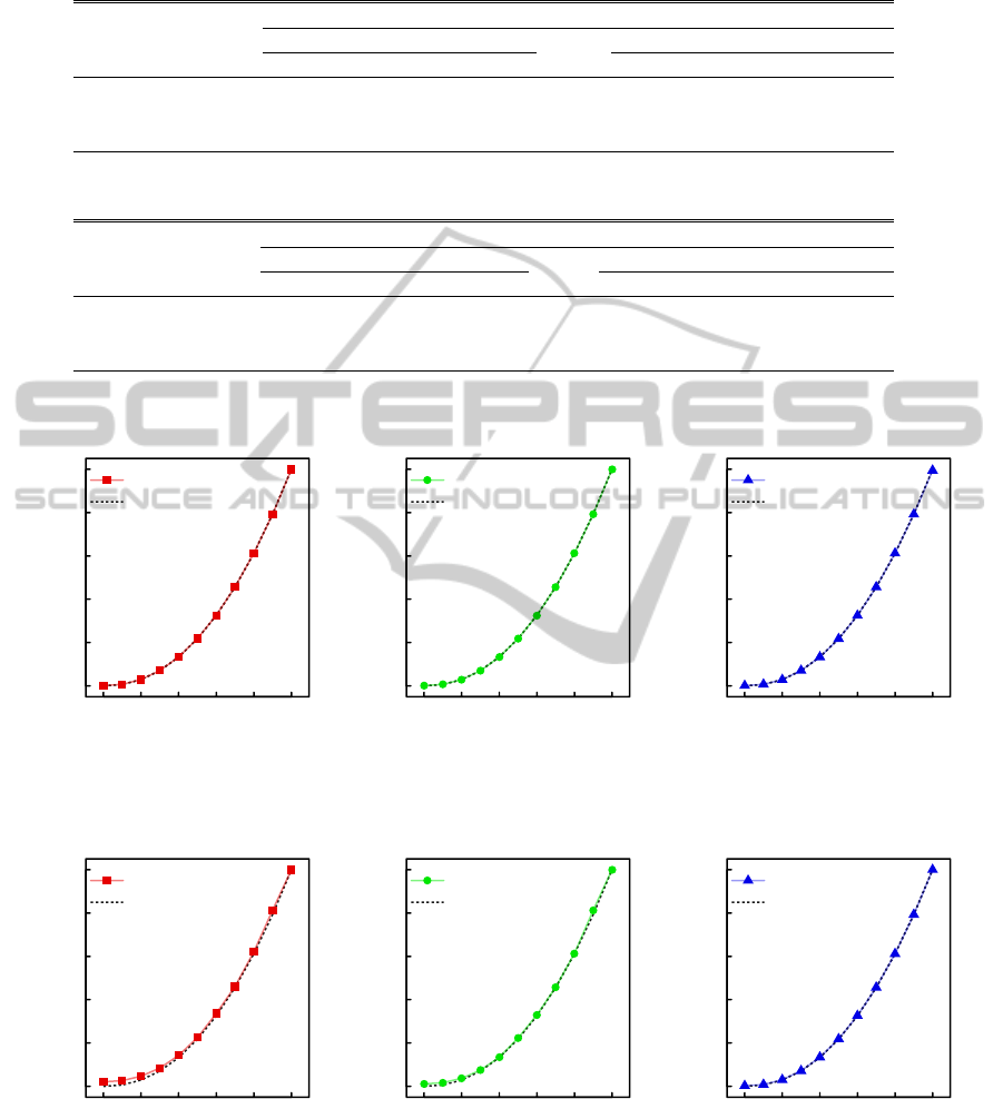
Table 2: Results of the errors in the spectral sensitivities recovered by the proposed method using synthetic data in the case of
nonlinear sensor responses (the gamma characteristic 2.2) under different noise levels.
RMSE of spectral sensitivity (×10
−5
)
Noise level Sony DXC-930 camera Kodak DCS-460 camera
R ch. G ch. B ch. R ch. G ch. B ch.
0.2% (σ = 0.002) 8.49 4.82 3.61 9.83 2.95 9.05
1% (σ = 0.01) 9.02 4.57 7.40 10.30 7.54 10.14
5% (σ = 0.05) 17.45 4.69 9.14 10.13 12.23 7.68
Table 3: The estimated standard deviation of sensor noise. The settings correspond to those in Table 2.
Absolute error of the estimated noise amount σ (×10
−3
)
Noise level Sony DXC-930 camera Kodak DCS-460 camera
R ch. G ch. B ch. R ch. G ch. B ch.
0.2% (σ = 0.002) 1.48 1.50 2.54 1.72 1.36 2.00
1% (σ = 0.01) 0.50 0.34 0.06 0.75 0.40 0.12
5% (σ = 0.05) 0.00 1.05 −0.60 −1.70 −0.35 0.20
(i) Sony DXC−930 camera
(ii) Kodak DCS−460 camera
0.0 0.4 0.8
0.0
0.2
0.4
0.6
0.8
1.0
Real sensor response
Linearized sensor response
recoverd
true
0.0 0.4 0.8
0.0
0.2
0.4
0.6
0.8
1.0
Real sensor response
Linearized sensor response
recoverd
true
0.0 0.4 0.8
0.0
0.2
0.4
0.6
0.8
1.0
Real sensor response
Linearized sensor response
recoverd
true
0.0 0.4 0.8
0.0
0.2
0.4
0.6
0.8
1.0
Real sensor response
Linearized sensor response
recoverd
true
0.0 0.4 0.8
0.0
0.2
0.4
0.6
0.8
1.0
Real sensor response
Linearized sensor response
recoverd
true
0.0 0.4 0.8
0.0
0.2
0.4
0.6
0.8
1.0
Real sensor response
Linearized sensor response
recoverd
true
R channel G channel B channel
R channel G channel B channel
Figure 3: Results of the estimated linearization functions. The settings correspond to those in Table 2.
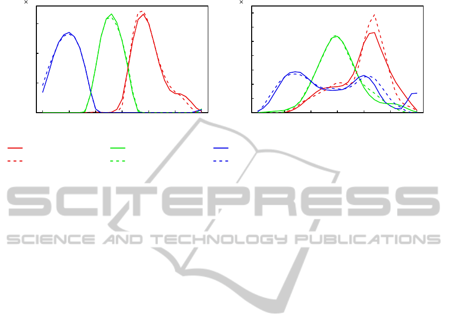
amounts were in the correct order. At last we show
the results of the spectral sensitivities recovered by
the proposed method in the presence of 1% sensor
noises for reference.
4 CONCLUSIONS
We proposed a Bayesian method for identifying cam-
era characteristics from an acquired image of a color
BayesianEstimationofCameraCharacteristicsincludingSpectralSensitivitiesfromaColorChartImagewithoutManual
ParameterTuning
21

400 450 500 550 600 650 700
0.0
0.5
1.0
1.5
Wavelength [nm ]
Sensitivity [a.u.]
10
- 3
400 450 500 550 600 650 700
0.0
0.2
0.4
0.6
0.8
1.0
1.2
1.4
Wavelength [nm ]
Sensitivity [a.u.]
10
- 3
R channel (recovered)
R channel (true)
G channel (recovered)
G channel (true)
B channel (recovered)
B channel (true)
Sony DXC−930 camera Kodak DCS−460 camera
Figure 4: Results of the spectral sensitivities by the proposed method. Nonlinear camera model (the gamma characteristic
2.2) are used and 1% noise (σ = 0.01) was added to the synthetic sensor response data.
chart. The key features are that it can obtain the
linearization function and the noise variance of each
color channel as well as the spectral sensitivity func-
tion, and never requires any manual tunings of param-
eters. The experiments using synthetic data demon-
strated high accuracy of the proposed method in re-
covering spectral sensitivities and linearization func-
tions. It was also found that the proposed method was
widely adaptable to the forms of sensitivity curves
and the levels of sensor noise. Experimental perfor-
mance tests are the next step of this study.
REFERENCES
Aronov, B., Asano, T., Katoh, N., Mehlhorn, K., and
Tokuyama, T. (2006). Polyline fitting of planar points
under min-sum criteria. International Journal of Com-
putational Geometry & Applications, 16:96–116.
Barnard, K. and Funt, B. V. (2002). Camera characteriza-
tion for color research. Color Research and Applica-
tion, 27(3):153–164.
Bishop, C. M. (2006). Pattern Recognition and Ma-
chine Learning (Information Science and Statistics).
Springer-Verlag New York, Inc., Secaucus, NJ, USA.
Carvalho, P., Santos, A., and Martins, P. (2004). Recovering
imaging device sensitivities: a data-driven approach.
Image Processing, 2004. ICIP ’04. 2004 International
Conference on, 4:2411–2414.
Finlayson, G., Hordley, S., and Hubel, P. M. (1998). Recov-
ering device sensitivities with quadratic programming.
Sixth Color Imaging Conference: Color Science, Sys-
tems and Applications, pages 90–95.
Grossberg, M. D. and Nayar, S. K. (2006). What can be
known about the radiometric response from images?
In Heyden, A., Sparr, G., Nielsen, M., and Johansen,
P., editors, Computer Vision – ECCV 2002, volume
2353 of Lecture Notes in Computer Science, pages
189–205. Springer Berlin Heidelberg.
Murayama, Y. and Ide-Ektessabi, A. (2012). Application of
bayesian image superresolution to spectral reflectance
estimation. Optical Engineering, 51:111713.
Sharma, G. and Trussell, H. (1997). Figures of merit for
color scanners. Image Processing, IEEE Transactions
on, 6(7):990–1001.
Sharma, G. and Trussell, H. J. (1996). Set theoretic esti-
mation in color scanner characterization. Journal of
Electronic Imaging, 5(4):479–489.
Shen, H.-L. and Xin, J. H. (2006). Spectral characteriza-
tion of a color scanner based on optimized adaptive
estimation. J. Opt. Soc. Am. A, 23(7):1566–1569.
Urban, P. and Grigat, R.-R. (2009). Metamer density esti-
mated color correction. Signal, Image and Video Pro-
cessing, 3:171–182.
Urban, P., Rosen, M., and Berns, R. (2008). A spatially
adaptive wiener filter for reflectance estimation. Final
Program and Proceedings - IS&T/SID Color Imaging
Conference, pages 279–284.
Vora, P. L., Farrell, J. E., Tietz, J. D., and Brainard,
D. H. (1997). Linear models for digital cameras. In
Proceedings, IS&T’s 50th Annual Conference, pages
377–382.
Zhao, H. Spectral sensitivity database. http://www.cvl.iis.u-
tokyo.ac.jp/ zhao/database.html.
VISAPP2013-InternationalConferenceonComputerVisionTheoryandApplications
22