
Color Quantization via Spatial Resolution Reduction
Giuliana Ramella and Gabriella Sanniti di Baja
Institute of Cybernetics "E.Caianiello", CNR, Via Campi Flegrei 34, Pozzuoli, Naples, Italy
Keywords: Color Quantization, Image Scaling, Voronoi Diagram.
Abstract: A color quantization algorithm is presented, which is based on the reduction of the spatial resolution of the
input image. The maximum number of colors n
f
desired for the output image is used to fix the proper spatial
resolution reduction factor. This is used to build a lower resolution version of the input image with size n
f
.
Colors found in the lower resolution image constitute the palette for the output image. The three
components of each color of the palette are interpreted as the coordinates of a voxel in the 3D discrete
space. The Voronoi Diagram of the set of voxels corresponding to the colors of the palette is computed and
is used for color mapping of the input image.
1 INTRODUCTION
Color quantization is a process that reduces the
number of distinct colors present in an input image
in such a way to originate a transformed image with
a noticeably smaller number of colors and at the
same time still visually similar to the input image.
One of the main applications of color quantization is
for image compression, especially when dealing
with the transmission of multimedia data files. These
files may have rather large size, so that their
transmission may result difficult due to the
bandwidth restrictions of computer networks. Other
applications of color quantization are for image
display, and for color based indexing and retrieval
from image databases.
Color quantization methods can be roughly
divided in image independent and image dependent
methods, see (Brun and Trémeau, 2002), (Celebi,
2011). The former methods, e. g., (Paeth, 1990),
(Mojsilovic and Soljanin, 2001), are generally
efficient, but produce poor results since the
distribution of colors in the input image is not taken
into account. Image dependent methods generally
provide good results, but are a bit more expensive.
Image dependent methods can be divided in pre-
clustering methods, e.g., (Heckbert, 1982),
(Gervautz and Purgathofer, 1990), (Wu, 1992),
(Kanjanawanishkul and Uyyanonvara, 2005), and
post-clustering methods, e.g., (Ozdemir and Akarun,
2002), (Bing et al., 2004), (Kim and Kehtarnavaz,
2005), (Atsalakis and Papamarkos, 2006), (Chen et
al., 2008), (Ramella and Sanniti di Baja, 2010),
(Rasti et al., 2011), (Celebi 2011). Pre-clustering
methods determine only once the color palette by
using features derived from the image at hand. Post-
clustering methods define an initial palette and then
improve it by resorting to an iterative process.
Color quantization can be interpreted as a
clustering problem in the 3D space, where the three
axes are the three color channels and the points are
the colors of the input image. To perform
quantization, points are suitably grouped into
clusters. Then, for each cluster a representative color
is selected, which is obtained e.g., as the average of
the points in the cluster. The number of clusters, i.e.,
the number of quantized colors, is generally fixed a
priori.
In principle, for a 24-bit true color image I the
number of possible colors may reach 16 millions.
However, the maximum number of colors actually
present in an image consisting of r rows and c
columns is rc. For example, consider an image I
with size 10241024. For such an image, at most
1.048.576 different colors are possible. In general, a
considerably smaller number of colors exists, since
the same color is likely to appear more than just
once in the image. On the other hand, if the spatial
resolution of I is reduced, say to 256256, a
maximum of 65.536 colors will be possible for its
pixels.
By taking into account the above considerations,
we here present a new image dependent technique
for color quantization that can be framed among the
78
Ramella G. and Sanniti di Baja G..
Color Quantization via Spatial Resolution Reduction.
DOI: 10.5220/0004272100780083
In Proceedings of the International Conference on Computer Vision Theory and Applications (VISAPP-2013), pages 78-83
ISBN: 978-989-8565-47-1
Copyright
c
2013 SCITEPRESS (Science and Technology Publications, Lda.)
pre-clustering methods. The method consists of two
processes, respectively dealing with the detection the
representative colors and with color mapping.
To find the representative colors, we resort to
spatial resolution reduction. This can be achieved by
any scaling down method. We use a classical
interpolation method (Pratt, 2001) and compute the
proper reduction factor that will allow us to build the
lower resolution image having the desired size. The
reduction of the spatial resolution of the input image
automatically implies an upper limit to the number
of colors in the palette.
During the second process, the Voronoi Diagram
is computed and is then used for color mapping.
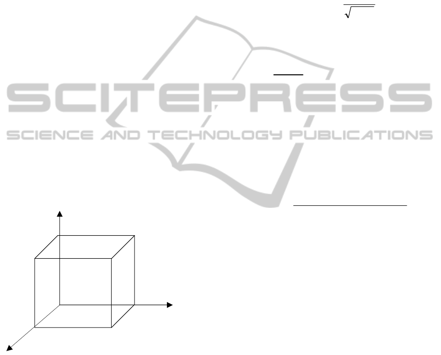
2 NOTIONS
Let I be an RGB color image. We interpret colors as
three-dimensional vectors, with each vector element
having an 8-bit dynamic range. We represent the
RGB color space as a 3D cube, where the three
coordinates of each point are the red, green and blue
components of that point in the color space, see
Figure 1. The edges of the cube have length 256,
since the values for the color components are in the
range [0, 255].
Figure 1: The 3D cube representing the RGB color space.
The color histogram of I can be built by reporting in
position (x, y, z) of the 3D cube the number of pixels
of I whose three color components have values x, y,
and z, respectively. The 3D histogram of colors
generally consists of a large and sparse set of points.
Since x, y, and z, as well as the value stored in
position (x, y, z) are integer numbers, the cube is a
discrete cube and we can refer to its points as to
voxels. Actually, we use a binary version of the 3D
histogram, where each voxel corresponding to an
existing color is set to 1, while all other voxels are
set to 0.
To evaluate the performance of our color
quantization algorithm, we use the Peak Signal to
Noise Ratio PSNR, the Structural SIMilarity SSIM,
the Colorloss CL, and the Compression Ratio CR.
For gray-level images, PSNR is computed as:
MSE
PSNR
255
log20
10
(1)
where
H
i
K
j
jiji
wv
KH
MSE
11
2
,,
1
(2)
and v
i,j
and w
i,j
respectively belong to the input
image and to the output image of size H×K.
For RGB images, the definition of PSNR is still
the same, but MSE is the sum over all squared value
differences divided by image size and by three.
The SSIM index for two gray-level images v and
w is computed as:
2
22
1
22
21
22
),(
cc
ccovc
wvSSIM
wvwv
vwwv
(3)
where μ
v
is the average of v; μ
w
is the average of w;
2
v
is the variance of v;
2
w
is the variance of w;
cov
vw
is the covariance of v and w; c
1
=(k
1
L)
2
and
c
2
=(k
2
L)
2
are two variables to stabilize the division
with weak denominator; L is the dynamic range of
the pixel values (255 for 8-bit image); and k
1
=0,01
and k
2
=0,03 are default values.
The SSIM index is computed within an 8×8
sliding window, which moves pixel-by-pixel from
top-left to bottom-right. As a result, an SSIM index
map of the image is obtained, and the overall quality
value is defined as the average of the SSIM index
map, i.e., the mean SSIM index. The value of SSIM
is in the range [0,1], where higher values denote
better structural similarity. For RGB images, the
SSIM index is computed for the three channel
components independently and the quality value is
obtained by the average of the three indexes.
The Colorloss CL is used to measure the loss of
color information caused by quantization. CL is
computed as the Euclidean color distance between a
pixel in the original image and the corresponding
B
Red (255, 0, 0)
Green (0, 255,0)
Blue (0,0,255) Magenta (255,0,255)
Yellow (255, 255, 0)
Cyan (0, 255, 255)
R
G
Black (0,0,
0)
White (255,255,255)
ColorQuantizationviaSpatialResolutionReduction
79

pixel in the quantized image. The loss in color
information increases with the colorloss. Let I
consist of N pixels, and let the RGB values of a pixel
p be (r
p
, g
p
, b
p
). Let I’ be the quantized image, where
q is the pixel corresponding to p with RGB values
(r
q
, g
q
, b
q
). Then, the average colorloss of a pixel
between these two images is defined as follows:
N
)()()(
)I CL(I,
1
222
N
qpqpqp
bbggrr
(4)
The compression ratio CR measures the percentage
of the original size of the image resulting after
compression. CR is computed as the ratio between
the size of the output stream and the input stream
expressed in bit per pixel (Salomon and Motta,
2010).
3 QUANTIZATION METHOD
Let I be the input color image with r
i
rows, c
i
columns and n
i
colors. Let n
f
be the maximum
number of colors desired for the quantized image.
To identify at most n
f
colors constituting the palette,
we reduce the spatial resolution of I so that the lower
resolution image is characterized by size equal to n
f
.
To this aim, we need to compute the proper value for
the reduction factor f.
The reduction factor is the ratio between the
number of rows r
f
(columns c
f
) that will characterize
the quantized image and the number of rows r
i
(columns c
i
) in the input image. Since it is:
fff
ncr
(5)
i
c
r
c
r
i
f
f
(6)
from which it results:
i
if
f
c
rn
r
(7)
we compute the reduction factor f that will originate
a lower resolution version of I including at most n
f
pixels and, hence, characterized by at most n
f
different colors.
Once the lower resolution image is available, it
includes at most n
f
different colors that constitute the
palette. The three components of the colors of the
palette are interpreted as coordinates of the only
voxels in a 256256256 cube, BH, that are set to 1.
Then, we perform connected component labeling, so
as to assign a different identity label to each
connected component of non zero voxels in BH.
Since some colors of the lower resolution image
may be very similar to each other, their
corresponding voxels in BH may be connected to
each other. Thus, the number of connected
components (and, hence, the number of final colors)
is likely to be smaller than the number of colors
existing in the lower resolution image. If connected
components including more than one voxel exist, for
any such a component the centroid is computed and
is used as representative color for the component.
The 3D Voronoi Diagram, where seeds consist of
connected components of voxels instead of
consisting of single voxels, is computed to divide
BH into as many Voronoi cells as many seeds have
been detected. To this aim, distance transformation
with identity label propagation is accomplished from
the seeds on the zero voxels of BH, by extending to
3D the algorithm suggested in (Fischler and Barrett,
1980) for the 2D case. In this way, the zero voxels of
BH are assigned the identity label of the seed to
which they are closer. All voxels in the same
Voronoi cell are associated the color of the
corresponding seed.
The quantized version of I is built during an
inspection of I. Each pixel p of I, whose color
components have values x, y, and z respectively,
receives the color associated to the Voronoi cell
including the voxel in position (x, y, z).
4 EXPERIMENTAL RESULTS
We have tested the quantization method on about
100 color images with different size and color
distribution, taken from available repositories (e. g.,
http://www.hlevkin.com/,http://sipi.usc.edu/database
/,http://r0k.us/graphics/kodak,http://www.eecs.berke
ley.edu/Research/Projects/CS/vision/bsds/). A small
set of six test images is shown in Figure 2.
The performance of our method can be
appreciated quantitatively by referring to Table 1,
where the results for the six test images are
summarized. For each test image, PSNR, SSIM, CL
and CR are computed for the quantized images
obtained in correspondence with different values of
n
f
, namely n
f
= 512, n
f
= 256, n
f
= 128, and n
f
= 64.
The value r
f
c
f
is also indicated, as well as the
number of final colors N
d
.
VISAPP2013-InternationalConferenceonComputerVisionTheoryandApplications
80
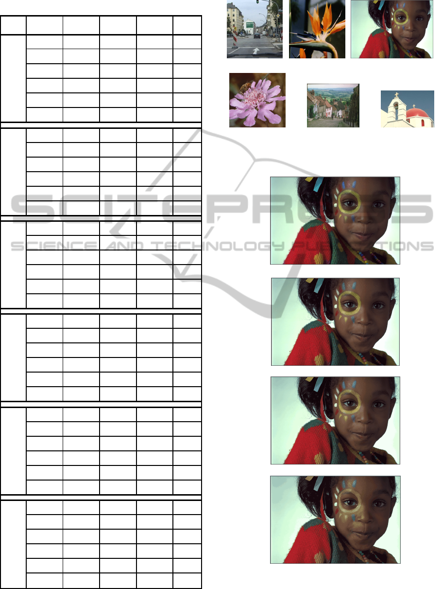
Table 1: Results for the six test images.
image n
f
=512 n
f
=256 n
f
=128 n
f
=64
1)
r
f
c
f
2222 1515 1111 88
N
d
418 210 117 63
SSIM 0.97 0.96 0.95 0.93
PSNR 37.53 35.33 33.88 32.05
CL 4.07 5.44 6.47 8.08
CR 0.57 0.50 0.45 0.39
2)
r
f
c
f
2222 1515 1111 88
N
d
406 204 116 63
SSIM 0.95 0.93 0.90 0.87
PSNR 36.84 34.15 31.98 29.44
CL 4.76 6.41 8.27 11.10
CR 0.54 0.47 0.42 0.37
3)
r
f
c
f
1827 1319 913 69
N
d
438 235 114 53
SSIM 0.96 0.95 0.93 0.89
PSNR 36.89 34.96 33.35 30.45
CL 4.18 5.44 7.00 10.15
CR 0.57 0.51 0.44 0.37
4)
r
f
c
f
2223 1516 1111 78
N
d
478 235 120 56
SSIM 0.96 0.94 0.92 0.88
PSNR 37.78 36.11 13.83 31.34
CL 4.41 5.49 7.18 9.74
CR 0.53 0.47 0.41 0.35
5)
r
f
c
f
2025 1417 912 79
N
d
458 230 105 63
SSIM 0.96 0.94 0.92 0.90
PSNR 36.53 34.50 31.87 30.46
CL 5.20 6.60 8.97 10.61
CR 0.53 0.47 0.40 0.36
6)
r
f
c
f
1827 1319 913 69
N
d
260 154 91 47
SSIM 0.98 0.97 0.96 0.94
PSNR 37.07 35.11 31.86 30.14
CL 2.98 3.78 5.40 7.70
CR 0.55 0.50 0.45 0.38
1) 512512, 42707 2) 512512, 73580 3) 512768, 44576
4) 480512, 111841 5) 384480, 111565 6) 312481, 31863
Figure 2: The six test images. For each image, the size and
the number of colors are given.
n
i
=44576
n
f
=256, N
d
=235
n
f
=128, N
d
=114
n
f
=64, N
d
=53
Figure 3: From top to bottom, the input image and
quantization results obtained by using different lower
resolution images.
ColorQuantizationviaSpatialResolutionReduction
81

To show qualitatively the performance of our
method, refer to Figure 3, where the results obtained
by using different lower resolution images to detect
the palette are shown for the test image 3).
Figure 4 shows the three lower resolution images
with n
f
= 256, n
f
= 128, and n
f
=64 respectively used
to obtain the three results given in Figure 3.
1319
913
69
Figure 4: From left to right, the lower resolution images
used to obtain the results shown in Figure 3. Pixel size has
been increased for visualization purposes.
The quantization method is easy to implement and
computationally advantageous. The results are
generally satisfactory. Of course, we are aware of
the limits of our approach. One drawback is that if n
f
is set to a small value (less than 64), the quality of
the resulting quantized image decreases
significantly. This is due to the fact that the value of
n
f
conditions the size of the lower resolution image.
If such a size is very small, the lower resolution
image is not adequate to represent the input image in
a satisfactory way.
Another drawback that can affect the method is
that colors characterized by large occurrence in the
input image, but forming regions with small size
(say, smaller than the size of the cells of the
decimation grid used by scaling down), are likely to
be not considered as colors of the palette.
We are working on possible solutions to alleviate
the above problems.
As for the first drawback, if the desired n
f
is very
small, the following process can be done. Instead of
computing a lower resolution image with size n
f
, we
build a lower resolution image with a larger size,
regarded as adequate for a satisfactory
representation of the input image and use it to fix the
palette. If the number of colors of the palette is
larger than n
f
, then colors that are sufficiently close
are clustered before computing the Voronoi
Diagram.
As for the second drawback, once the lower
resolution image has been generated, the palette is
enriched by adding colors that, though characterized
in the original image by large occurrence, do not
exist in the lower resolution image.
5 CONCLUDING REMARKS
A new color quantization algorithm has been
presented, which is based on the detection of the
representative colors in a lower resolution version of
the input color image. The maximum number of
desired colors is used to fix the reduction factor and
build the lower resolution image. Colors found in the
lower resolution image are taken as seeds for the
computation of the Voronoi Diagram. Colors of the
input image in the same Voronoi cell are associated
the color of the corresponding seed.
REFERENCES
Atsalakis, A., Papamarkos, N., 2006. Color reduction and
estimation of the number of dominant colors by using
a self-growing and self-organized neural gas,
Engineering Applications of Artificial Intelligence 19,
769-786.
Bing, Z., Junyi, S., Qinke, P., 2004. An adjustable
algorithm for color quantization, Pattern Recognition
Letters
25, 1787–1797.
Brun, L., Trémeau, A., 2002.
Digital Color Imaging
Handbook
, Chapter 9: Color Quantization, 589–638,
Electrical and Applied Signal Processing, CRC Press.
Celebi, M. E., 2011. Improving the performance of k-
means for color quantization,
Image and Vision
Computing
29, 260–271, 2011.
Chen, T. W., Chen, Y. L. Chien, S. Y., 2008. Fast image
segmentation based on K-means clustering with
histograms in HSV color space, Proc. IEEE 10th
Workshop on Multimedia Signal Processing
, 322-325.
Fischler, M. A., Barrett, A., 1980. An iconic transform for
sketch completion and shape abstraction, Computer
Graphics and Image Processing
13, 334-360.
VISAPP2013-InternationalConferenceonComputerVisionTheoryandApplications
82

Gervautz, M., W. Purgtathofer, W., 1990. A Simple
Method for Color Quantization:Octree Quantization.
San Diego, CA, Academic.
Heckbert, P. S., 1982. Color Image Quantization for
Frame Buffer Display,
ACM SIGGRAPH '82 16(3),
297-307.
Kanjanawanishkul, K., Uyyanonvara, B., 2005. Novel fast
color reduction algorithm for time-constrained
applications,
Journal of Visual Communication and
Image Representation
16, 311–332.
Kim, N., Kehtarnavaz, N., 2005. DWT-based scene-
adaptive color quantization, Real-Time Imaging 11,
443–453.
Mojsilovic, A., Soljanin E., 2001. Color quantization and
processing by Fibonacci lattices, IEEE Transactions
on Image Processing 10 (11), 1712–1725.
Ozdemir, D., Akarun, L., 2002. A fuzzy algorithm for
color quantization of images,
Pattern Recognition 35,
1785–1791.
Paeth, A. W., 1990. Mapping RGB triples onto four bits,
in A. S. Glassner, Ed.,
Graphics Gems, Academic
Press, Cambridge, MA, 233–245.
Pratt, W. K., 2001. Digital Image Processing, John Wiley
& Sons, New York.
Ramella, G., Sanniti di Baja, G., 2010. Multiresolution
histogram analysis for color reduction,
Proc. 15th
Iberoamerican Congress on Pattern Recognition
, eds.
I. Bloch, M.R. Cesar-Jr., LNCS 6419, Springer,
Berlin, 22-29.
Rasti, J., Monadjemi, A., Vafaei, A., 2011. Color
reduction using a multi-stage Kohonen Self-
Organizing Map with redundant features,
Expert
Systems with Applications
38, 13188–13197.
Salomon, D., Motta, G., 2010.
Handbook of Data
Compression
, Springer, Fifth Edition.
Wu, X., 1992. Color quantization by dynamic
programming and principal analysis, ACM
Transactions on Graphics
11/4, 349-372.
ColorQuantizationviaSpatialResolutionReduction
83
