
Probabilistic View-based 3D Curve Skeleton Computation on the GPU
Jacek Kustra
1,3
, Andrei Jalba
2
and Alexandru Telea
1
1
Institute Johann Bernoulli, University of Groningen, Nijenborgh 9, Groningen, The Netherlands
2
Eindhoven University of Technology, Den Dolech 2, Eindhoven, The Netherlands
3
Philips Research, Eindhoven, The Netherlands
Keywords:
Curve Skeletons, Stereo Vision, Shape Reconstruction, GPU Image Processing.
Abstract:
Computing curve skeletons of 3D shapes is a challenging task. Recently, a high-potential technique for this
task was proposed, based on integrating medial information obtained from several 2D projections of a 3D
shape (Livesu et al., 2012). However effective, this technique is strongly influenced in terms of complexity by
the quality of a so-called skeleton probability volume, which encodes potential 3D curve-skeleton locations.
In this paper, we extend the above method to deliver a highly accurate and discriminative curve-skeleton
probability volume. For this, we analyze the error sources of the original technique, and propose improvements
in terms of accuracy, culling false positives, and speed. We show that our technique can deliver point-cloud
curve-skeletons which are close to the desired locations, even in the absence of complex postprocessing. We
demonstrate our technique on several 3D models.
1 INTRODUCTION
Curve skeletons are well-known 3D shape descriptors
with applications in computer vision, path planning,
robotics, shape matching, and computer animation.
A 3D object admits two types of skeletons: Surface
skeletons are 2D manifolds which contain the loci
of maximally-inscribed balls in a shape (Siddiqi and
Pizer, 2009). Curve skeletons are 1D curves which
are locally centered in the shape (Cornea et al., 2005).
Curve skeleton extraction has received increased
attention in the last years (Dey and Sun, 2006; Re-
niers et al., 2008; Jalba et al., 2012; Au et al., 2008;
Ma et al., 2012; Tagliasacchi et al., 2009; Cao et al.,
2010a; Tagliasacchi et al., 2012). All these meth-
ods work in object space, i.e. take as input a 3D
shape description coming as a voxel model, mesh, or
dense point cloud. Recently, Livesu et al. have pro-
posed a fundamentally different approach: They ex-
tract the curve skeleton from a set of 2D views of a
3D shape (Livesu et al., 2012). Key to this compu-
tation is the extraction of a volume which encodes, at
each 3D point inside the shape, the probability that the
curve-skeleton passes through that point. The curve-
skeleton is extracted from this volume using a set of
postprocessing techniques. This approach has the ma-
jor advantage that it requires only a set of 2D views
of the input shape, so it can be used when one does
not have a complete 3D shape model. However, this
method strongly depends on the quality of the skeletal
probability volume.
We present here an extension of the view-based
approach of Livesu et al., with the following contri-
butions. First, we propose a different way for com-
puting the curve-skeleton probability and represent-
ing it as a dense point cloud. On the one hand, this
eliminates a major part of the original proposal’s false
positives (i.e., locations where a curve-skeleton point
is suggested, but no such point actually exists), which
makes our probability better suited for further skele-
ton extraction. On the other hand, our point-cloud
model eliminates the need for a costly voxel repre-
sentation. Secondly, we propose a fast GPU imple-
mentation of the point cloud computation which also
delivers the skeleton probability with higher accuracy
than the original method. We demonstrate our tech-
nique on several complex 3D models.
The structure of this paper is as follows. Section 2
overviews related work on 3D curve skeleton extrac-
tion. Section 3 details the three steps of our frame-
work: extraction of accurate 2D view-based skeletons
(Sec. 3.1), a conservative stereo matching for extract-
ing 3D skeleton points from 2D view pairs, (Sec. 3.2),
and a sharpening step that delivers a point cloud nar-
rowly condensed along the curve skeleton (Sec. 3.3).
Section 4 presents several results and discusses our
237
Kustra J., Jalba A. and Telea A..
Probabilistic View-based 3D Curve Skeleton Computation on the GPU.
DOI: 10.5220/0004276502370246
In Proceedings of the International Conference on Computer Vision Theory and Applications (VISAPP-2013), pages 237-246
ISBN: 978-989-8565-48-8
Copyright
c
2013 SCITEPRESS (Science and Technology Publications, Lda.)

framework. Section 5 concludes the paper.
2 RELATED WORK
2.1 Preliminaries
Given a three-dimensional binary shape Ω ⊂ R
3
with
boundary ∂Ω, we first define its distance transform
DT
∂Ω
: Ω → R
+
as
DT
∂Ω
(x ∈ Ω) = min
y∈∂Ω
∥x −y∥ (1)
The surface skeleton of Ω is next defined as
S
∂Ω
= {x ∈ Ω|∃f
1
,f
2
∈ ∂Ω,f
1
̸= f
2
,
∥x − f
1
∥ = ∥x − f
2
∥ = DT
∂Ω
(x)}, (2)
where f
1
and f
2
are two contact points with ∂Ω of
the maximally inscribed disc in Ω centered at x, also
called feature transform (FT) points (Strzodka and
Telea, 2004) or spoke vectors (Stolpner et al., 2009).
Here, the feature transform is defined as
FT
∂Ω
(x ∈ Ω) = argmin
y∈∂Ω
∥x − y∥. (3)
Note that FT
∂Ω
is multi-valued, as an inscribed ball
can have two, or more, contact points f. Note, also,
that the above definitions for the distance transform,
feature transform, and skeleton are also valid in the
case of a 2D shape Ω ∈ R
2
.
2.2 Object-space Curve Skeletonization
In contrast to the formal definition of surface skele-
tons (Eqn. 2), curve skeletons know several defini-
tions in the literature. Earlier methods computed the
curve skeleton by thinning, or eroding, the input voxel
shape in the order of its distance transform, until a
connected voxel curve is left (Bai et al., 2007). Thin-
ning can also be used to compute so-called meso-
skeletons, i.e. a mix of surface skeletons and curve
skeletons (Liu et al., 2010). For mesh-based models,
a related technique collapses the input mesh along its
surface normals under various constraints required to
maintain its quality (Au et al., 2008). Hassouna et
al. present a variational technique which extracts the
skeleton by tracking salient nodes on the input shape
in a volumetric cost field that encodes centrality (Has-
souna and Farag, 2009). Tagliassacchi et al. com-
pute curve skeletons as centers of point cloud projec-
tions on a cut plane found by optimizing for circular-
ity (Tagliasacchi et al., 2009). A good review of curve
skeletonization is given in (Cornea et al., 2007).
One of the first formal definitions of curve skele-
tons is the locus of points x ∈ Ω which admit at least
two shortest paths, or geodesics, between their fea-
ture points (Dey and Sun, 2006; Prohaska and Hege,
2002). This definition has been used for mesh mod-
els (Dey and Sun, 2006) and voxel-based models (Re-
niers et al., 2008). Curve skeletons can also be ex-
tracted by collapsing a previously computed surface
skeleton towards its center using differents variants
of mean curvature flow (Tagliasacchi et al., 2012;
Cao et al., 2010a; Telea and Jalba, 2012). Alterna-
tively, surface skeletons can be computed using a ball
shrinking method (Ma et al., 2012) and then select-
ing points which match the geodesic criterion (Jalba
et al., 2012). However, such approaches require one
to first compute the more expensive surface skeleton.
2.3 View-based Curve Skeletonization
A quite different approach was recently proposed by
Livesu et al.: Noting that the 2D projection of a 3D
curve skeleton is close to the 2D skeleton of the pro-
jection, or view, of an input 3D shape, they extract
curve skeletons by merging 2D skeletal information
obtained from several views of the input shape Ω.
Given two such views C
i
and C
⊥
i
, whose up-vectors
are parallel and lines of sight are orthogonal, the sil-
houettes B
i
and B
⊥
i
of Ω are first computed by orto-
graphic projection of the input shape. Secondly, the
2D skeletons S
∂B
i
and S
∂B
⊥
i
of these silhouettes are
computed. Next, stereo vision is used to reconstruct
the 3D skeleton: Point pairs p ∈ S
B
i
and p
⊥
∈ S
B
⊥
i
are
found by scanning each epipolar line, and then back-
projected into 3D to yield a potential curve-skeleton
point x
1
. The points x found in this way are accu-
mulated into a so-called probability volume V ⊂ R
3
,
which gives, at each spatial point, the likelihood to
have a curve-skeleton passing through that point.
The above method has several advantages com-
pared to earlier techniques. First, it can be used di-
rectly on shape views, rather than 3D shape models,
which makes it suitable for any model which can be
rendered in a 2D view, regardless of its representa-
tion (e.g. polygons, splats, points, lines, or textures).
Secondly, the method can be easily parallelized, as
view pairs are treated independently. However, this
method fundamentally relies on the fast computation
of a good probability volume which contains a correct
estimation of the curve skeleton location. This poses
the following requirements:
1. a reliable and accurate stereo vision correspon-
1
Here and next, we denote by italics (e.g., p) the 2D
projection of a 3D point p in a camera C
VISAPP2013-InternationalConferenceonComputerVisionTheoryandApplications
238

dence matching, i.e. finding the correct pairs of
points (p ∈ S
∂B
i
, p
⊥
∈ S
∂B
⊥
i
) which represent the
projection of the same curve skeleton point in the
view-pair (C
i
,C
⊥
i
);
2. an accurate and efficient representation of the
probability volume V for further processing.
Requirement (1) is not considered by Livesu et al.,
where all possible point-pairs along an epipolar line
are backprojected. This generates, as we shall see in
Sec. 3.2.2, a large amount of noise in the probabil-
ity volume V . Removing this noise requires four rel-
atively complex postprocessing steps in the original
proposal. Secondly, the probability volume V is rep-
resented as a voxel grid. This makes the method un-
necessarily inaccurate, relatively slow and hard to par-
allelize, and requires large amounts of memory, thus
contradicts requirement (2).
In the following, we present several enhancements
that make view-based skeleton extraction compatible
with requirements (1) and (2). This allows us to ex-
tract a high-accuracy probability volume for further
usage in curve skeleton computation or direct visual-
ization.
3 ACCURATE PROBABILITY
VOLUME COMPUTATION
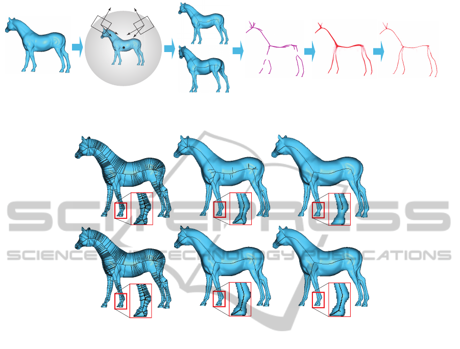
Our proposal has three steps (see also Fig. 1).
First, we extract regularized and subpixel-accuracy
2D skeletons from several views of the input shape
(Sec. 3.1). Next, we use additional view-based infor-
mation to infer a conservative set of correspondences
between points in such 2D skeleton pairs, backpro-
ject these in 3D, and record the obtained points as a
point cloud (Sec. 3.2). Finally, we apply an additional
sharpening step on the 3D point cloud, which directly
delivers a highly accurate curve-skeleton probability
(Sec. 3.3).
3.1 Robust 2D Skeletonization
Given a shape Ω and camera specification C =
(o,v,u) described by its origin o, view direction v,
and up-vector u, we start by computing the silhou-
ette B of Ω by rendering the shape on the camera’s
view plane (u,v ×u). Next, we compute the so-called
salience 2D skeleton of B using the technique pre-
sented in (Telea, 2012a). The salience of a point p ∈ B
is defined as
σ(p) =
ρ(p)
DT
∂B
(p)
(4)
Here, DT
∂B
(p) is the 2D distance transform of the sil-
houette boundary ∂B and ρ(p) is the so-called skele-
ton importance
ρ(p) = max
f
1
,f
2
∈FT
∂B
(p)
∥γ
f
1
f
2
∥ (5)
where FT
∂B
is the feature transform of the boundary
∂B, and γ
ab
is the compact boundary fragment be-
tween two points a and b on ∂B. The importance ρ
increases monotonically from the endpoints (tips) of
the skeleton towards its center. Intuitively, ρ(p) as-
sociates, to each skeleton point p, the length of the
longest boundary arc (in pixels) subtended by its fea-
ture points. Upper thresholding ρ with a value ρ
0
will
thus remove both skeleton branches created by small
boundary wiggles and end-parts of important skeleton
branches caused e.g. by boundary corners. Figure 2
(top row) shows this effect for a silhouette B of a horse
model. For ρ
0
= 1, we get the full 2D skeleton, which
contains many spurious branches. For ρ
0
= 5, we get
the desired skeleton detail at the legs and head, but
still have several spurious branches around the rump
and neck. For ρ
0
= 30, we eliminate all spurious
branches, but also loose relevant portions of branches
corresponding to the legs. This is undesired, since, as
we shall later see, we need the important branches at
their full length to reconstruct a curve-skeleton reach-
ing into all shape protrusions.
In contrast, the salience metric σ (Eqn. 4) deliv-
ers a better result. As shown in (Telea, 2012a), σ
is high along the most important, or salient, skeleton
branches, and low elsewhere. Hence, we can thresh-
old σ to obtain the skeleton
S
∂B
= {p ∈ B|σ(p) > σ
0
} (6)
Equation 6 delivers a clean, regularized, skele-
ton whose spurious branches are eliminated, and
whose important branches extend all the way into the
shape’s protrusions. Figure 2 (bottom row) shows the
saliency-based regularization. For σ
0
= 0, we obtain
the same full skeleton as for ρ
0
= 1. Increasing σ
0
over a value of 0.05 practically removes all spurious
branches, but keeps the important ones un-pruned (see
zoom-ins). As such, we use the value σ
0
= 0.05 fur-
ther in our pipeline.
We further enhance the precision of the com-
puted skeleton by using the subpixel technique pre-
sented in (Strzodka and Telea, 2004). As such, skele-
ton points are stored as 2D floating-point coordinates
rather than integers. This will be important when per-
forming the 3D stereo reconstruction (Sec. 3.2.2).
3.2 Accurate Correspondence Matching
We find potential 3D curve-skeleton points along the
same key idea of (Livesu et al., 2012): Given a cam-
ProbabilisticView-based3DCurveSkeletonComputationontheGPU
239
input 3D shape Ω
C
⊥
C
u
v
o
v
⊥
u
⊥
o
⊥
camera-pair
selection
silhouette
skeletonization
S
S
⊥
pair matching+culling
and 3D backprojection
silhouette and
depth culling
3D skeleton
sharpening
Figure 1: Curve-skeleton probability computational pipeline.
σ
0
=0 σ
0
=0.05 σ
0
=0.1
ρ
0
=0
ρ
0
=5
ρ
0
=30
Figure 2: Skeleton regularization. Top row: Importance-based method (Telea and van Wijk, 2002) for three different threshold
values ρ
0
. Bottom row: Salience-based method (Telea, 2012a) for three different threshold values σ
0
.
era C = (o, v,u), where v points towards the object’s
origin, we construct a pair-camera C
⊥
= (o
⊥
,v
⊥
,u
⊥
)
which also points at the origin and so that the two up-
vectors u and u
⊥
are parallel. In this case, projected
points p in C correspond to projected points p
⊥
in C
⊥
located on the same horizontal scanline. Given such
a point-pair (p,p
⊥
), the generated 3D point x is com-
puted by triangulation, i.e. by solving
x = p + kv = p
⊥
+ k
⊥
v
⊥
(7)
where p and p
⊥
are the 3D locations, in their respec-
tive view planes, corresponding to p and p
⊥
respec-
tively, and k and k
⊥
are the distances between x and
the view planes of C and C
⊥
. Note that p and p
⊥
can
be immediately computed as we know the positions
of p and p
⊥
and the cameras’ positions, orientations,
and near plane locations.
3.2.1 Correspondence Problem
However, as well known in stereo vision, the suc-
cess of applying Eqn. 7 is fundamentally conditioned
by having the correct 2D points p and p
⊥
paired in
the two cameras. Let us analyze this issue in our
context: Consider that a scanline y intersects a 2D
skeleton shape in m points on the average. Hence,
we have m
2
possible point-pairs. These will gener-
ate m
2
points in the 3D reconstruction, whereas in
reality there are only at most m such points – that
is, if no occlusion is present. The excess of m
2
− m
points are false positives. Given N such camera-pairs
placed uniformly around the object in order to re-
construct its 3D curve skeleton, and considering a
camera viewplane of P × P pixels, we have in the
worst case O(N(m
2
− m)P) false-positive points in
the curve skeleton. The ratio of false-to-true posi-
tives is thus Π = O
(
N(m
2
− m)P)/(NmP)
)
= O(m).
In our measurements for a wide set of shapes, we no-
ticed that m = 5 on the average. Concretely, at an
image resolution of P
2
= 1024
2
pixels, and using the
setting N = 21 from Livesu et al., we thus get over
400K false-positive points generated in excess of the
NPm ≃ 100K true-positive skeleton points.
The above false-to-true-positive ratio Π is a con-
servative estimate: Given a rigid shape Ω, the 2D
skeleton of its silhouette can change considerably as
the silhouette changes, even when no self occlusions
occur. This, and additional self-occlusion effects, re-
VISAPP2013-InternationalConferenceonComputerVisionTheoryandApplications
240

duce the true-positive count and thus increases Π.
This ultimately creates substantial noise in the curve-
skeleton probability estimation, and thus makes an ac-
curate curve skeleton extraction more complex.
3.2.2 Pair-culling Heuristic
We reduce the false-to-true-positive ratio Π by using
additional information present in our cameras, as fol-
lows. Consider a point p on a scanline L in C and all
points L
⊥
= {p
⊥
i
} on the same scanline in C
⊥
(see
Fig. 3 e). The 3D reconstructions of all pairs (p, p
⊥
i
)
lie along the line p+ kv (Eqn. 7). Hence, if we had an
estimate of the depth k
est
between the correct recon-
struction and the viewplane of C, we could select the
best pair p
⊥
est
for p as
p
⊥
est
= argmin
p
⊥
est
∈L
⊥
|k
est
− k| (8)
i.e. the point in C
⊥
which yields, together with p,
a depth closest to our estimate. We estimate k
est
as follows: When we draw the shape in C, we also
compute its nearest and furthest depth buffers Z
n
and
Z
f
, by rendering the shape twice using the OpenGL
GL LESS and GL GREATER depth-comparison func-
tions respectively. Next, for each point p in the
viewplane of C, we set k
est
=
1
2
[Z
n
(p) + Z
f
(p)] (see
Fig. 3 e).
It is essential to note that our heuristic for k
est
is
not an attempt to find the exact value of the depth
k. Indeed, if we could do this, we would not need
to apply Eqn. 8, as we could perform the 3D back-
projection using a single view. We use k
est
only as a
way to select the most likely point-pair for 3D recon-
struction. This is argumented as follows: First, we
note that the value k for the correct point-pair must
reside between Z
n
(p) and Z
f
(p) - indeed, the recon-
structed 3D point x must be inside the object’s hull.
Secondly, the curve skeleton is roughly situated in the
(local) middle of the object, thus its depth is close to
k
est
. Thirdly, we note that, when the angle between
the cameras’ vectors α = ∠(v,v
⊥
) decreases, then the
depths k
i
yielded by Eqn. 8 for a set of scanline-points
p
⊥
i
∈ L
⊥
get further apart. In detail, if the distance be-
tween two neighbor pixels in the scanline L
⊥
is δ, the
distance between their reconstructions using the same
point p in the other scanline L is ε = δ/ sin(α), see
Fig. 3 c. Hence, if we use a small α (under 90
deg
),
we get fewer depths k
i
close to k
est
, so we decrease
the probability that selecting the point whose depth is
closest to k
est
(Eqn. 8) will yield an incorrect point-
pair for the 3D reconstruction. In contrast, Livesu et
al. use α = 90
◦
, as this slightly simplifies Eqn. 7.
Given that low α values reduce the likelihood to ob-
tain false pairs using our depth heuristic, we prefer
this, and set α = 20
◦
.
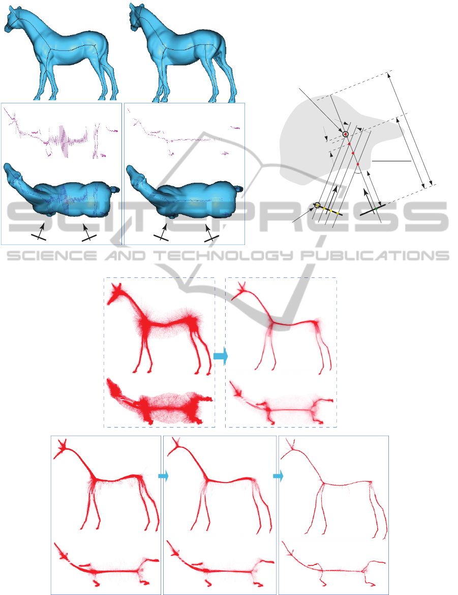
Figure 3 shows the results of using our depth-
based pairing heuristic. Images (a) and (b) show
the two skeletons S
∂B
and S
∂B
⊥
corresponding to the
two cameras C and C
⊥
respectively. The brute-force
many-to-many correspondence pairing yields 6046
three-dimensional points. As visible in Fig. 3 c,
these points are spread uniformly in depth along the
view directions of the two cameras. This is expected,
since 2D skeleton pixels are equally spaced in the im-
age plane. For clarity, we displayed here only those
points which pass the silhouette and depth-culling, i.e.
which are inside the object from any considered view
(see further Sec. 3.3). The displayed points in Fig. 3 c
are thus final points in the curve-skeleton probability
volume delivered by many-to-many matching.
Figure 3 d shows the reconstructed 3D points
when we use our depth-based pair-culling. Since
we now only have one-to-one pairs, we obtain much
less points (721 vs 6046, see the explanations in
Sec. 3.2.1). Moreover, these points are located very
close to the actual curve skeleton, as shown by the
top view of the model.
Given our conservative point-pair selection, as
shown in Fig. 4, we generate much fewer curve-
skeleton points than if using many-to-many pairing.
Although this is highly desirable for obtaining an
accurate (false-positive-free) curve skeleton, it also
means that the curve skeleton will be sparser than
when using all possible pairs. To counteract this, we
simply use more view pairs N. In practice, setting
N ≃ 500 yields sufficiently dense curve skeletons (see
results in Sec. 4). An additional advantage of using
more views is that we do not need to carefully select
the optimal views for stereo reconstruction, in con-
trast to the original method, where such views are ob-
tained by performing a principal component analysis
(PCA) on both the 3D shape and its 2D projections.
We further reduce the number of tested point-pairs
(Eqn. 8) by scanning L from left to right (for p) and
L
⊥
from right to left (for p
⊥
), As such, 3D points
are generated in increasing order of their depth k, so
|k
est
− k| first decreases, then increases. Hence, we
stop the scan as soon as |k
est
− k| increases, which
gives an additional speed improvement.
3.3 Probability Sharpening
We collect the 3D points x (Eqn. 7) found by the
depth-based correspondence matching for a given
camera-pair (C,C
⊥
) in an unstructured point cloud
C S . As C rotates around the input shape, we keep
testing that the projections x of the accumulated
ProbabilisticView-based3DCurveSkeletonComputationontheGPU
241
d) pair culling: 721 pairs
a) first view (C)
b) second view (C
⊥
)
c) full pairing: 6046 pairs
C C
⊥
v
⊥
v
C C
⊥
v
⊥
v
C
scanline L
⊥
v
⊥
v
p
p
i
⊥
α
e) pair matching and triangulation
skeleton pixel
resolution
δ
depth spread ε
scanline L
shape Ω
Z
f
(p)
Z
n
(p)
Z
n
(p)+Z
f
(p)
2
reconstructed
point x
selected p
⊥
est
Figure 3: Correspondence matching for curve-skeleton reconstruction. A camera pair (a,b). Reconstructed 3D points when
using full pairing (c) and when using our depth-based pairing (d). Depth-based pairing and triangulation (e).
a) original density volume b) density volume (low opacity)
c) pair culling
d) depth culling
e) sharpening
2599632 points
242689 points258899 points 253081 points
2599632 points
Figure 4: Curve-skeleton probability point-cloud. (a) original method (Livesu et al., 2012). (b) Cloud in (a) displayed with
lower opacity. (c) Effect of depth-based pairing. (d) Effect of depth culling. (e) Effect of sharpening (see Sec. 3.3).
VISAPP2013-InternationalConferenceonComputerVisionTheoryandApplications
242

points x ∈ C S fall inside the silhouette B in C, as
well as within C’s depth range [Z
n
(x),Z
f
(x)]. Points
which do not pass these tests are eliminated from C S .
The depth test explained above comes atop the sil-
houette test which was already proposed by Livesu
et al.. Whereas the silhouette test constrains C S to
fall within the visual hull of our input shape, we con-
strain C S even further, namely to fall within the exact
shape. The difference is relevant for objects with cav-
ities, whose visual hull is larger than the object itself.
However closer to the true curve-skeleton than the
results presented by Livesu et al., our C S still shows
some spread around the location of the true curve
skeleton. This is due to two factors. First, consider
the inherent variability of 2D skeletons in views of a
3D object: The 2D skeleton is locally centered with
respect to the silhouette (or projection) of a 3D object
Ω. In areas where Ω has circular symmetry, the 2D
skeleton of the projected 3D object is indeed identi-
cal to the 2D projection of the true 3D curve skele-
ton, i.e., skeletonization and projection are commuta-
tive. However, this is not true in general for shapes
with other cross-sections. Moreover, self-occlusions,
in the case of concave objects, will generate 2D skele-
tons which have little in common with the projection
of the curve skeleton. It is important to stress that
this is not a problem caused by wrong correspondence
matching. Secondly, using a small α angle between
the camera pairs (Sec. 3.2.2), coupled with the inher-
ent resolution limitations of the image-based skele-
tons, introduces some depth estimation errors which
show up as spatial noise in the curve skeleton.
We further improve the sharpness of C S as fol-
lows. For each camera C which generates a silhouette
B, we move the points x ∈ C S parallel to the view
plane of C with a step equal to ∇DT
∂B
. Since ∇DT
∂B
points towards S
∂B
, this moves the curve-skeleton
points towards the 2D skeleton S
∂B
. Note that, in gen-
eral, ∇DT
∂B
is not zero along S
∂B
(Telea and van Wijk,
2002). Hence, to prevent points to drift along S
∂B
, and
thus create gaps in the curve skeleton, we disallow
moving points x which already project on S
∂B
. Note
also that this advection nevers move points outside Ω,
since S
∂B
is always inside any sihouette B of Ω. Since
the above process is done for all the viewpoints C, the
curve skeleton gets influenced by all the considered
views. This is an important difference with respect to
Livesu et al., where a 3D skeleton point is determined
only by two views.
Figure 4 shows the effect of our three improve-
ment steps: depth-based pairing (Sec. 3.2.2), depth
culling, and sharpening. All images show 3D point
clouds rendered with alpha blending. Figure 4 a
shows the cloud C S computed following the orig-
inal method of Livesu et al., that is, with many-
to-many correspondence matching along scanlines
(Sec. 3.2.1). Clearly, this cloud contains a huge
amount of points not even close to the actual curve
skeleton. If we decrease the alpha value in the visu-
alization, we see that this cloud, indeed, has a higher
density along the curve-skeleton (Fig. 4 b). We see
here also that naive thresholding of the density, which
is quite similar to decreasing the alpha value to obtain
Fig. 4 b from Fig. 4 a, creates problems: If a too low
threshold is used, the skeleton still stays thick; if a too
high threshold is used, the skeleton risks disconnec-
tions (see white gaps in the neck region in Fig. 4 b).
Eliminating the large amount of false positives
from the cloud shown in Fig. 4 a is very challeng-
ing. To do this, Livesu et al. apply an involved
post-processing pipeline: (1) voxelize the cloud into
a voting grid; (2) extract a maximized spanning tree
(MST) from the grid; (3) detect and prune perceptu-
ally salient tree branches; (4) collapse short branches;
(5) recover curve-skeleton loops lost by the MST; and
(6) smooth the resulting skeleton; for details we re-
fer to (Livesu et al., 2012). Although this is possi-
ble, as demonstrated by the results of Livesu et al.,
this post-processing is highly complex, delicate, and
time-consuming.
Fig. 4 c shows our curve-skeleton probability,
obtained with the center-based correspondence pair
culling (Sec. 3.2.2). The point cloud contains now
around ten times less points. Also, note that points
close to the true curve skeleton have been well de-
tected, i.e., we also have few false negatives. Apply-
ing the depth-based culling further removes a small
amount of false positives (Fig. 4 d vs Fig. 4 c). Fi-
nally, the density sharpening step effectively attracts
the curve-skeleton points towards the local skeleton
in each view, so the overall result is a sharpening of
the point cloud C S , i.e. a point density increase along
the true curve skeleton and a density decrease further
from the skeleton (Fig. 4 e).
4 DISCUSSION
Performance. We have implemented our method
in
C++ with OpenGL and CUDA and tested it on a 2.8
GHz MacBook Pro with an Nvidia GT 330M graph-
ics card. The main effort is spent in computing the
regularized 2D salience skeletons (Sec. 3.1). We effi-
ciently implemented the computation of DT
∂B
, FT
∂B
,
ρ, and σ (Eqns. 1-4) using the method in (Cao et al.,
2010b), one of the fastest exact Euclidean distance-
and-feature transform techniques in existence (see our
ProbabilisticView-based3DCurveSkeletonComputationontheGPU
243
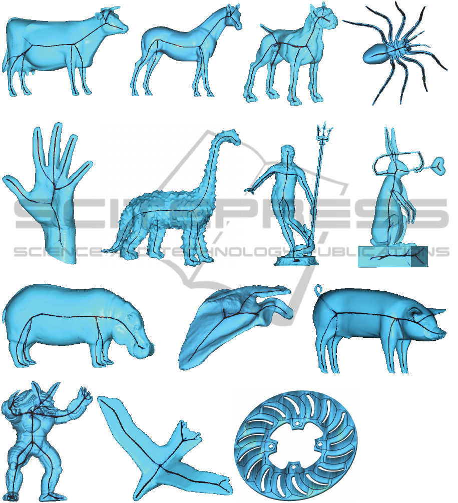
a) cow b) horse c) hound
d) spider
e) hand f) dino g) neptune h) rabbit
i) hippo j) scapula k) pig
l) armadillo m) bird n) rotor
Figure 5: Curve-skeleton probability point-clouds for several models (see Sec. 4).
publicly available code at (Telea, 2012b)). The re-
maining steps of our pipeline are trivial to paral-
lelize, as points and camera views are treated inde-
pendently. Overall, our entire pipeline runs roughly
at 500 frames/second. Given that we use more views
than Livesu et al., i.e. roughly 500 vs 21, our CUDA-
based parallelization is essential, as it allows us to
achieve roughly the same timings as the method of
Livesu et al.
Parameters. All parameters of the method are fixed
and independent on the input shape, i.e. skele-
ton saliency threshold σ
0
= 0.05 (Sec. 3.1), num-
ber of considered views uniformly distributed around
a sphere centered in the object center N = 500
VISAPP2013-InternationalConferenceonComputerVisionTheoryandApplications
244

a) b) c) d)
e) g)f)
Figure 6: Comparison with related methods: (a) our method; (b) (Livesu et al., 2012); (c) (Telea and Jalba, 2012); (d) (Au
et al., 2008); (e) (Dey and Sun, 2006); (f) (Jalba et al., 2012); (g) (Reniers et al., 2008) (see Sec. 4).
(Sec. 3.2.2), screen resolution P
2
= 1024
2
pixels
(Sec. 3.2.1), and angle between the camera-pair view
vectors α = 20
◦
(Sec. 3.2.2). Less views (N < 500)
will generate sparser-sampled curve skeletons, as dis-
cussed in Sec. 3.2.2. Decreasing the pixel resolution
generates slightly thicker point distributions in the
curve-skeleton cloud. This is expected, since we have
less and coarser-spaced 2D skeleton pixels, which
also implies higher depth estimation errors (Eqn. 7).
Decreasing α under roughly 5 degrees generates too
large inaccuracies in the depth estimation; increasing
it over roughly 30 degrees reduces the likelihood of
good correspondence pairing; hence, our setting of
α = 20
◦
.
Results. Figure 5 shows several results computed
with our method. The produced curve-skeleton
clouds contain between 100K and 300K points. We
render these clouds using small point splats of 2 by
2 pixels, to make them more visible. The key obser-
vation is that our skeleton point clouds are already
very close to the desired 3D location, even in the ab-
sence of any cloud postprocessing. In contrast, the
equivalent point clouds delivered by the method of
Livesu et al. are much noisier (see example in Fig. 3 a
and related discussion in Sec. 3.2.2), and thus require
significant postprocessing to select the true-positives.
Since our point clouds are much sharper, we can di-
rectly use them for curve-skeleton visualization, as
shown in Fig. 5. If an explicit line representation of
such skeletons is desired, this can be easily obtained
by using e.g. the curve-skeleton reconstruction algo-
rithm described in (Jalba et al., 2012), Sec. VIII-C.
Thin tubular skeleton representations can be obtained
by isosurfacing the density field induced by our 3D
point cloud. In this paper, we refrained from produc-
ing such reconstructions, as we want to let our main
contribution stand apart – the computation of noise-
free, accurate point-cloud representations of the curve
skeleton probability.
Comparison. Figure 6 compares our method with
several recent curve-skeleton extraction methods. As
visible, our curve skeleton has the same overall struc-
ture and positioning within the object. However, dif-
ferences exist. First, our method produces smoother
curve skeletons than (Dey and Sun, 2006) and (Jalba
et al., 2012). This is due to the density sharpen-
ing step, which does not have an equivalent in the
latter two methods. Also, (Au et al., 2008) re-
quires a so-called connectivity surgery step to re-
pair the curve skeleton after the main Laplacian ad-
vection has completed. This necessary step has the
undesired by-product of creating straight-line inter-
nal skeleton branches (Fig. 6 d, palm center). Sec-
ondly, we correctly find the skeleton’s ligature and
internal branches. This is also the case for all other
methods except (Livesu et al., 2012), where all skele-
ton branches are merged in a single junction point
(Fig. 6 b). This fact is not surprising, given the branch
collapsing postprocessing step in the latter method. It
is not clear to us why this step is required (or benefi-
cial), as it actually changes the topology of the skele-
ton, and thus may impair operations such as shape
analysis or matching.
Properties. Our method maintains all of the desir-
able properties of curve skeletons advocated by re-
lated work (Cornea et al., 2007; Au et al., 2008;
Tagliasacchi et al., 2012; Livesu et al., 2012; Jalba
et al., 2012): Our skeletons are thin and locally cen-
tered within the object. Higher-genus objects (with
tunnels) are handled well (see rabbit and rotor mod-
els, Fig. 5). The method is robust against noise, due
to the sharpening step (see dino and armadillo mod-
els, Fig. 5). Thin, sharp detail protrusions of the mod-
els generate curve skeleton branches, as long as these
parts project to at least 1 pixel in screen space (see
neptune, spider, and rabbit models, Fig. 5). This is
due to the usage of the 2D skeleton saliency metric,
which keeps 2D skeleton branches reaching into such
salient shape details (Sec. 3.1). Input model resolu-
tion, e.g. polygon count, is largely irrelevant to the
end result, since 2D skeletons are computed in image
space.
Limitations. Our method cannot recover complete
curve skeletons for shape parts which are not visible
from any viewpoint, i.e., permanently self-occluded.
This is an inherent problem of view-based 3D recon-
ProbabilisticView-based3DCurveSkeletonComputationontheGPU
245

struction. For such shapes, the object-space skele-
tonization methods mentioned in Sec. 2 should be
used.
5 CONCLUSIONS
We have presented a new method for computing
curve-skeletons as unstructured point clouds. Our
method extends the view-based curve-skeleton ex-
traction of Livesu et al. in several directions: (1)
Using salience-based skeletons to guarantee preser-
vation of terminal skeleton branches, (2) using depth
information to reduce the number of false-positives in
the 3D skeleton reconstruction, and (3) sharpening the
obtained point-cloud representation to better approx-
imate the 1D singularity locus of the curve skeleton.
We trade off speed for accuracy, by generating more
conservative skeleton samples and using more view-
points. However, by using a GPU implementation,
we achieve the same speed as the original method,
but deliver a much cleaner and sharper 3D skeleton
point-cloud approximation. Overall, our method can
be used either as a front-end for reconstructing line-
based representations of 3D curve skeletons, or for di-
rectly rendering such skeletons as unstructured point
clouds.
Future work can improve the point matching ac-
curacy, for example by using optical flow models
or exploiting geometric variability properties of 2D
skeletons. Separately, implementing the 3D geodesic-
based curve-skeleton detector of (Dey and Sun, 2006)
by using the 2D collapsed boundary metric ρ (Eqn. 5)
is a promising way for recovering highly accurate
curve skeletons in this view-based framework.
REFERENCES
Au, O. K. C., Tai, C., Chu, H., Cohen-Or, D., and Lee, T.
(2008). Skeleton extraction by mesh contraction. In
Proc. ACM SIGGRAPH, pages 441–449.
Bai, X., Latecki, L., and Liu, W.-Y. (2007). Skeleton prun-
ing by contour partitioning with discrete curve evolu-
tion. IEEE TPAMI, 3(29):449–462.
Cao, J., Tagliasacchi, A., Olson, M., Zhang, H., and Su,
Z. (2010a). Point cloud skeletons via laplacian-based
contraction. In Proc. IEEE SMI, pages 187–197.
Cao, T., Tang, K., Mohamed, A., and Tan, T. (2010b). Paral-
lel banding algorithm to compute exact distance trans-
form with the GPU. In Proc. SIGGRAPH I3D Symp.,
pages 134–141.
Cornea, N., Silver, D., and Min, P. (2007). Curve-skeleton
properties, applications, and algorithms. IEEE TVCG,
13(3):87–95.
Cornea, N., Silver, D., Yuan, X., and Balasubramanian, R.
(2005). Computing hierarchical curve-skeletons of 3D
objects. Visual Comput., 21(11):945–955.
Dey, T. and Sun, J. (2006). Defining and computing curve
skeletons with medial geodesic functions. In Proc.
SGP, pages 143–152. IEEE.
Hassouna, M. and Farag, A. (2009). Variational curve
skeletons using gradient vector flow. IEEE TPAMI,
31(12):2257–2274.
Jalba, A., Kustra, J., and Telea, A. (2012). Comput-
ing surface and curve skeletons from large meshes
on the GPU. IEEE TPAMI. accepted; see
http://www.cs.rug.nl/∼alext/PAPERS/PAMI12.
Liu, L., Chambers, E., Letscher, D., and Ju, T. (2010). A
simple and robust thinning algorithm on cell com-
plexes. CGF, 29(7):22532260.
Livesu, M., Guggeri, F., and Scateni, R. (2012). Re-
constructing the curve-skeletons of 3D shapes
using the visual hull. IEEE TVCG, (PrePrints). http://
doi.ieeecomputersociety.org/10.1109/TVCG.2012.71.
Ma, J., Bae, S. W., and Choi, S. (2012). 3D medial axis
point approximation using nearest neighbors and the
normal field. Visual Comput., 28(1):7–19.
Prohaska, S. and Hege, H. C. (2002). Fast visualization
of plane-like structures in voxel data. In Proc. IEEE
Visualization, page 2936.
Reniers, D., van Wijk, J. J., and Telea, A. (2008). Com-
puting multiscale skeletons of genus 0 objects using a
global importance measure. IEEE TVCG, 14(2):355–
368.
Siddiqi, K. and Pizer, S. (2009). Medial Representations:
Mathematics, Algorithms and Applications. Springer.
Stolpner, S., Whitesides, S., and Siddiqi, K. (2009). Sam-
pled medial loci and boundary differential geometry.
In Proc. IEEE 3DIM, pages 87–95.
Strzodka, R. and Telea, A. (2004). Generalized distance
transforms and skeletons in graphics hardware. In
Proc. VisSym, pages 221–230.
Tagliasacchi, A., Alhashim, I., Olson, M., and Zhang, H.
(2012). Skeletonization by mean curvature flow. In
Proc. Symp. Geom. Proc., pages 342–350.
Tagliasacchi, A., Zhang, H., and Cohen-Or, D. (2009).
Curve skeleton extraction from incomplete point
cloud. In Proc. SIGGRAPH, pages 541–550.
Telea, A. (2012a). Feature preserving smoothing of shapes
using saliency skeletons. Visualization in Medicine
and Life Sciences, pages 155–172.
Telea, A. (2012b). GPU skeletonization code.
www.cs.rug.nl/svcg/Shapes/CUDASkel.
Telea, A. and Jalba, A. (2012). Computing curve skeletons
from medial surfaces of 3d shapes. In Proc. Theory
and Practice of Computer Graphics (TPCG), pages
224–232. Eurographics.
Telea, A. and van Wijk, J. J. (2002). An augmented fast
marching method for computing skeletons and center-
lines. In Proc. VisSym, pages 251–259.
VISAPP2013-InternationalConferenceonComputerVisionTheoryandApplications
246
