Supply Chain Risk Assessment Applying System Dynamics Approach

Case Study: Apparel Industry

Marzieh Mehrjoo and Zbigniew J. Pasek

Department of Industrial and Manufacturing Systems Engineering, University of Windsor, Windsor, Canada

Keywords: Supply Chain, Risk Assessment, System Dynamics, Simulation, Apparel Industry.

Abstract: A remarkable increase in the demand and supply uncertainty, as the primary sources of supply chain risk

and other sources such as: capacity constraints, supply variability, parts quality problems, long lead times,

war and natural disasters have increased the necessity of assessing and managing the risk in the supply

chain. The purpose of this study is to investigate the impact of two categories of risk, demand uncertainty

and delays, on the performance of an apparel supply chain. A system dynamics approach was used to study

the behavior and relationships within the supply chain of this industry. The proposed model facilitates the

study and identification of the critical components of the supply chain. In addition, the model provides a

tool to generate multiple business scenarios for effective decision making.

1 INTRODUCTION

Uncertainty in the demand for products is the

primary source of risk in the supply chain. Several

interdependent factors such as higher product

variety, shorter product life cycles, increased

customer expectations, more complex and longer

supply chains, and more global competitions have

increased this uncertainty considerably in the recent

years. Moreover, capacity constraints, supply

variability, parts quality problems, long lead times,

and manufacturing yields besides disruptions due to

war and natural disasters are some other sources of

risks in the supply chain (Sheffi and Rice, 2005).

Therefore, it is essential for companies to understand

supply chain interdependencies, identify potential

risk factors, their likelihood and consequences

(Tummala and Schoenherr, 2011). They need to

develop plans for disruptions and contingency plans

to decrease the likelihood of supply chain risks.

In the apparel industry, market demand is highly

volatile and product life cycles are short. Low

predictability and high level of impulse purchase are

other characteristics of this market (Carugati et al.,

2008). All the previously mentioned factors increase

the importance of risk assessment for the supply

chain of these products. Barlas and Aksogan (1997)

built a system dynamics simulation model for the

textile and apparel pipeline which consisted of

wholesaler and retailer levels. They studied the

effects of product diversity and quick response order

strategies on customer demand, possible stockouts

and inventory levels.The purpose of this study is to

investigate the impact of two categories of risks -

demand uncertainty and delays - on the performance

of an apparel supply chain through a system

dynamics approach.

2 MODEL

Industrial dynamics (Forrester, 1961) introduced a

methodology for the simulation of dynamic models,

which is the origin of system dynamics (Sterman,

2000). Extensive research in various fields, natural

and social sciences, has been conducted using

system dynamics. System dynamics is one of the

best methods for analyzing complex systems

(Campuzano and Mula, 2011). In this study, the

system dynamics software, Vensim®, was used as a

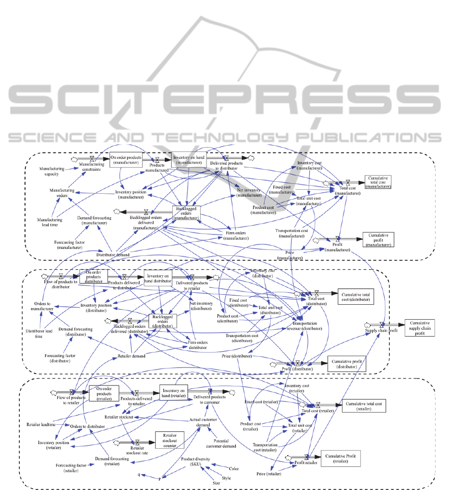
tool to build the supply chain model. The model (see

Fig. 5) has three primary members: a manufacturer,

a distributor and a retailer.

At the retailing level for an apparel store, when

the customer’s need is not satisfied, the customer

usually leaves and does not wait for his/her need to

be fullfilled. Therefore, the constructed model has

considered the orders not delivered on time as the

lost sale at this stage. If the warehouse contains the

sufficient amount of products to meet the demand at

343

Mehrjoo M. and Pasek Z..

Supply Chain Risk Assessment Applying System Dynamics Approach - Case Study: Apparel Industry.

DOI: 10.5220/0004276601450148

In Proceedings of the 2nd International Conference on Operations Research and Enterprise Systems (ICORES-2013), pages 145-148

ISBN: 978-989-8565-40-2

 2013 SCITEPRESS (Science and Technology Publications, Lda.)

the time, the order is delivered. Otherwise, the final

customer’s demand is transferred to increase the

“Retailer stockout” variable. Based on the inventory

position, forecasted demand and lead time of this

stage, the retailer’s replenishment orders will be sent

to the distributor through the “Orders to distributor”

variable. The output of “On order products

(retailer)” is “Products delivered to retailer” which is

affected by the lead time and introduces a delay into

the arrival of products. The delay is considered to be

pure and not exponential, that means that the arrival

of products at the warehouse happens exactly after

the period defined in the “Retailer lead time”

variable.

At the distributor level, if the orders are not met

by the required date, they will be served when the

distributor has enough stock available. The proposed

model considered the orders not delivered on time as

backlogged orders and they were included in the

daily firm orders. The flow of information and

material at the distributor level undergoes the same

transformations as the previous level except the case

of backlogged orders that do not exist in the retailing

level.

The service and delivery policies for backlogged

or delayed orders at the manufacturer level follow

the same formulation as the distributor level. The

manufacturer has a predefined daily capacity, so it

can only manufacture the amount of units the factory

is capable of.

The demand forecasts are calculated during each

period based on a simple exponential smoothing

technique.

In the proposed model, the total cost is calculated

based on the unit cost, the amount of products

delivered including delivered backlogged orders,

products manufactured for the manufacturer level

and products purchased for the other two stages. It is

assumed that the distributor is the member

responsible for all the transportations taking place in

the supply chain. Therefore, the variables of

“transportation revenue” and the “transportation

cost” are included in this level. It should be

mentioned that a variable to calculate the total

revenue of each stage is not defined separately, but it

is calculated inside the formula of the profit variable.

In order to test the validity of the model, three

different tests including direct extreme conditions

test, dimentional consistency test and direct structure

test, by comparing the model equations with

available knowledge in the literature, were

conducted.

The main characteristics of the model including

model parameters and assumptions are as follows:

 It is possible to serve only one part of the

order when the whole order is not available.

 Inventory management is performed applying

inventory review policy.

 The raw materials used for manufacturing are

considered to be available all the time.

 Simulation takes place over 365 periods.

 The stock of the initial inventory for the

manufacturer level is 10 units and for both,

distributor and retailer, are 5 units.

 The manufacturing capacity is 25 units per

period.

 The manufacturing lead time is 8 periods and

the manufacturing lead time to the distributor

and then to the retailer are 2 and 1 periods,

respectively.

 The adjust factor for forecasting is equal to 2.

 The pattern selected for the number of

customers entering the retail store per period

corresponds to a normal distribution with the

μ = 25 and σ = 9.

 Since a customer who enters the store may

leave without buying an item, a binomial

distribution was selected to calculate the

probability that a customer will prefer a SKU

in the retail store.

 Actual customer’s demand is calculated by

multiplication of the number of customers

entering the retail store and the probability

that a customer will buy an item after

entering the store.

 Number of color, style and size varieties of

products are 5, 12 and 10, respectively.

3 RISK ASSESSMENT

As mentioned previously, this paper studies the

effect of demand variability and the risk of delay on

the supply chain performance of an apparel industry.

The cumulative cost in each stage of the supply

chain is used as the performance measure.

3.1 Risk of Delay

In order to investigate the impact of delay, four

different scenarios have been considered. In the

Main scenario there is no increase in the lead time of

any of the stages; in LT1 there are 6 periods of time

increase only in the lead time of manufacturer; in

LT2 there are 5 periods of time increase only in the

lead time of distributor; and in LT3 there are 2 units

of time increase only in the lead time of the retailer.

Figures 1 to 3 depict the results of the simulation. It

ICORES2013-InternationalConferenceonOperationsResearchandEnterpriseSystems

344

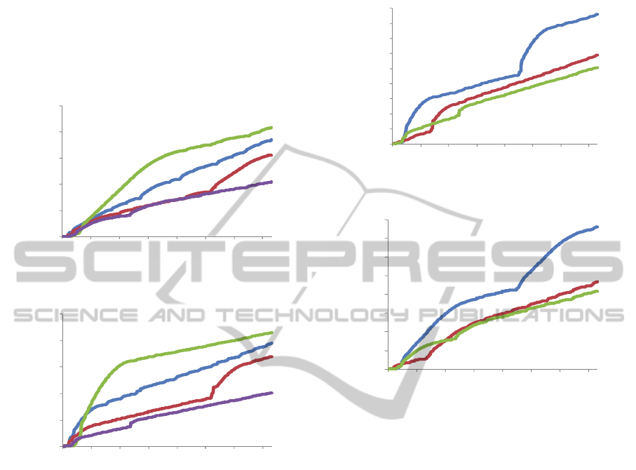
can be seen that the Main scenario, with no delay in

the model, has the least cost in all the three stages of

the supply chain. Also, delay in the lead time of

manufacturer level, LT1, causes the highest cost

increase in the manufacturing and distribution

stages. The costs in the retailing stage are mainly

sensitive to the delays in the same stage, retailing

(not shown).

Figure 1: Effect of delay in lead time on manufacturer

cumulative total cost.

Figure 2: Effect of delay in lead time on distributor

cumulative total cost.

3.2 Risk of Demand Variability

Three scenarios were defined to compare the

performance of the supply chain under various

variabilities of demand patterns. The number of

customers entering the retailing store (potential

customer demand) follows a normal distribution

with the following characteristics

 Main: Range = 40 and σ = 9,

 Dem 1: Range = 40 and σ = 25.

 Dem 2: Range = 90 and σ = 9.

From Fig. 3, it can be interpreted that increasing the

variation of demand has a higher impact on the

manufactuer and distributor compared to the retailer,

considerably increasing their costs. In addition, these

two stages perform worse when the data related to

the demand comes from an interval with longer

width (Fig. 4). In the designed supply chain, the

retailer stage shows the least sensitivity to the

variation and uncertainty in demand.

Figure 3: Effect of demand variability on manufacturer

cumulative total cost.

Figure 4: Effect of demand variability on distributor

cumulative total cost.

4 SUMMARY

This paper presented a system dynamics model that

can be used to study and observe the processes and

relationships in the supply chain of an apparel

industry. It is also useful as a high-level tool to

analyze the impact of different types of risks

associated with the supply chain of this industry.

This study investigated the impact of demand

uncertainty and risk of delay on the supply chain

performance. The main limitation of the model is the

data used as the inputs. Due to the inability to obtain

more accurate industry-specific data, the absolute

numbers that this model presented are used for

comparative analysis of different scenarios.

Nevertheless, the model helps to study the

relationships between supply chain stages and to

analyze the effect of changing values for the

variables of the model.

10000

20000

30000

40000

50000

0 50 100 150 200 250 300 350

CumulativeTotalCost(Mfg.)[$]

Time[periods]

LT1

LT3

LT2

main

50000

100000

150000

200000

250000

0 50 100 150 200 250 300 350

CumulativeTotalCost(Distr.)[$]

Time [periods]

LT1

LT3

LT2

main

20000

40000

60000

80000

100000

120000

140000

160000

180000

0 50 100 150 200 250 300 350

CumulativeTotalCost(Distr.) [$]

Dem1

Dem2

main

Time [periods]

5000

10000

15000

20000

25000

30000

35000

40000

0 50 100 150 200 250 300 350

CumulativeTotalCost(Mfg.)[$]

Dem1

Dem2

main

Time [days]

SupplyChainRiskAssessmentApplyingSystemDynamicsApproach-CaseStudy:ApparelIndustry

345

REFERENCES

Barlas, Y., Aksogan, A., 1997. Product Diversification and

Quick Response Order Strategies in Supply Chain

Management. Available from

http://ieiris.cc.boun.edu.tr/faculty/barlas.

Campuzano, F. and Mula, J., 2011. Supply Chain

Simulation: A System Dynamics Approach for

Improving Performance. Springer London Dordrecht

Heidelberg New York.

Carugati, A., Liao, R., Smith, P., 2008. Speed-to-Fashion:

Managing Global Supply Chain in Zara. Proceedings

of the IEEE ICMIT, pp. 1494-1499.

Choi, T.Y. Krause, D.R., 2006. The supply base and its

complexity: implications for transaction costs, risks,

responsiveness, and innovation. Journal of Operations

Management, Vol. 24 No. 5, pp. 637-52.

Forrester, J.W., 1961. Industrial Dynamics. MIT Press and

Wiley, New York.

Sheffi, Y., Rice Jr., J.B., 2005. A Supply chain view of the

resilient enterprise. MIT Sloan Management Review,

Vol. 47 No. 1., pp. 41-48.

Sterman, J.D., 2000. Business Dynamics: Systems

Thinking and Modeling for a Complex World.

McGraw-Hill Higher Education, New York.

Tummala, R., Schoenherr, T., 2011. Assessing and

managing risks using the Supply Chain Risk

Management Process (SCRMP). Supply Chain

Management: An International Journal, Vol. 16 No. 6,

pp. 474–483.

Zsidisin, G.A., Ellram, L.M., Carter, J.R. Cavinato, J.L.,

2004. An analysis of supply risk assessment

techniques. International Journal of Physical

Distribution & Logistics Management, Vol. 34 No. 5,

pp. 397-409.

Zsidisin, G.A., Panelli, A., Upton, R. 2000. Purchasing

organization involvement in risk assessments,

contingency plans, and risk management: an

exploratory study. Supply Chain Management: An

International Journal, Vol. 5 No. 4, pp. 187-97.

APPENDIX

Figure 5: The stock flow diagram of an apparel supply chain using Vensim software.

Retailer

Distributor

Manufactu

ICORES2013-InternationalConferenceonOperationsResearchandEnterpriseSystems

346