
Directable Animation of Non-photorealistic Fluids
Viraj Churi, Gaurav Bhagwat and Parag Chaudhuri
Department of Computer Science and Engineering, Indian Institute of Technology Bombay, Mumbai, India
Keywords:
Physically-based Fluid Simulation, Stroke-based Interface, Directable Fluids, Non-photorealistic Rendering.
Abstract:
This paper presents a method to control and direct a physically-based fluid simulation with user defined
strokes. Strokes are interpreted as flowlines and introduce a smooth velocity field in their vicinity that allows
the fluid simulation to be easily directed by an animator. We also allow the fluid to interact with arbitrarily
shaped obstacles and have variable viscosity during the simulation. The strokes can be alive for a finite du-
ration and are registered to a timeline to give keyframing like control to the animator over the physics driven
simulation.
1 INTRODUCTION
Traditionally trained animators trying to create spe-
cial effects animation for fluids in two-dimensions
have to be very skilled artists to capture the flow of
energy that makes the movement of fluids convincing
(Gilland, 2009). On the other hand, recent research
in graphics (Stam, 1999; Foster and Fedkiw, 2001;
Batty et al., 2007) has made physically-based simu-
lation of fluids accessible to all. However, physics
driven fluids, though mathematically realistic are of-
ten too cumbersome to control and direct for artists
who cannot parse the various parameters that have to
be adjusted to fine-tune the simulation. Thus, there is
a need for intuitive controls for fluid animation that
let artists direct the fluid behavior easily.
Our paper describes a stroke-based control
method for directing the animation of fluids. We han-
dle fluids in two-dimensions as we want to enhance
and ease the work of animators trained in the 2D do-
main. The strokes drawn by the artist act as flowlines
and the fluid is guided along these strokes. An ex-
ample of these can be seen in Figure 1. The strokes
are a natural interface for the artist used to sketching
and drawing. Our fluid simulation is an Eulerian grid
based technique that uses a combination of fluid im-
plicit particle (FLIP) method and particle in cell (PIC)
method to advect the fluid (Zhu and Bridson, 2005).
We further use the variational method for the pressure
solve to achieve one-way solid-fluid coupling (Batty
et al., 2007). This lets us handle obstacles of arbitrary
shape in the simulation.
The rest of this paper is organized as follows. We
discuss related prior work and our basic fluid simula-
tion framework in Section 2. We describe our stroke-
based interface for directing the fluid in Section 3,
additional controls for the fluid simulation in Sec-
tion 4 and our non-photorealistic renderer details in
Section 5. We conclude by summarizing our results
in Section 6 and the contributions of this paper, its
limitations and outlining avenues for future work in
Section 7.
2 BACKGROUND
We briefly review related works in grid-based
fluid simulation, controlling fluid flows and non-
photorealistic rendering of fluids.
2.1 Fluid Simulation
(Foster and Metaxas, 1996) introduced the first 3D
grid-based solver for fluid simulation to computer
graphics. This was followed by the stable fluids work
of (Stam, 1999) who used Semi-Lagrangian advec-
tion to obtain unconditional stability in the simulator.
(Foster and Fedkiw, 2001) used a level set for higher
quality tracking of the fluid surface. Subsequently,
(Zhu and Bridson, 2005) used a combination of PIC
and FLIP techniques for particle advection while sim-
ulating sand as a fluid. More recent work also intro-
duce fully implicit methods for computing two-way
interactions between solids and fluids that offer better
accuracy and stability (Chentanez et al., 2006; Batty
et al., 2007). We are inspired by these works in creat-
ing our basic fluid simulation framework.
254
Churi V., Bhagwat G. and Chaudhuri P..
Directable Animation of Non-photorealistic Fluids.
DOI: 10.5220/0004277402540260
In Proceedings of the International Conference on Computer Graphics Theory and Applications and International Conference on Information
Visualization Theory and Applications (GRAPP-2013), pages 254-260
ISBN: 978-989-8565-46-4
Copyright
c
2013 SCITEPRESS (Science and Technology Publications, Lda.)
(a) (b) (c) (d) (e)
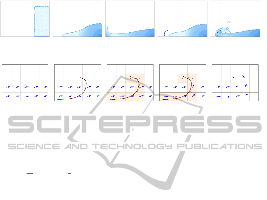
Figure 1: (a), (b) and (c) show a normal dam break simulation. (d) shows a stroke added to the frame shown in (b). This
changes the resulting splash wave in the dam break simulation as shown in (e).
(a) (b) (c) (d) (e)
Figure 2: (a)-(b) A velocity stroke is introduced in flow (drawn in red). (c)-(d) The cells through which the stroke passes
are identified and the flow velocity in those cells is changed to match the tangent vectors on the stroke. This causes the flow
direction to get locally modified to match the stroke. (e) Subsequent advection steps smooth out the velocity field and spread
the stroke induced velocities to nearby cells.
We solve the Navier-Stokes equations for incom-
pressible fluid flows as given below, on a staggered
grid.
∂u
∂t
+ (u · ∇u)u +
1
ρ
∇p = f (1)
∇ · u = 0 (2)
Here u is the fluid velocity, ρ the fluid density, p is
the pressure, and f is the acceleration due to body
forces such as gravity. Interested readers can refer
to (Bridson, 2008) for more details on the standard
grid-based fluid solver. We use the pressure solve re-
formulated as a kinetic energy minimization (Batty
et al., 2007). This allows us to robustly handle
solid-fluid interactions. We track a signed distance
function by using the fast sweeping algorithm (Zhao,
2004) for computing the numerical solution of the
Eikonal equation. This is used to reconstruct a smooth
fluid surface at higher grid resolutions using marching
squares (Lorensen and Cline, 1987). The grid resolu-
tion used for surface tracking can be controlled using
the surface refinement factor that can be 1, 2 or 4 with
higher numbers signifying a more refined grid.
2.2 Controlling Fluid Flows
Control of fully 3D fluid simulation was attempted
early on where embedded controllers were used for
altering pressure and velocity in the fluid (Foster
and Metaxas, 1997). (Rasmussen et al., 2004) use
particle-based controls for velocity, viscosity, level-
sets and divergence. (McNamara et al., 2004) use
the adjoint method to efficiently solve the non-linear
optimization problem involved in matching the con-
trol parameters to user defined keyframes. (Mihalef
et al., 2004) present a slice based control mechanism
to specify the keyframes of breaking waves. (Th
¨
urey
et al., 2006) present a control mechanism in which
control particles locally exert forces in the fluid to
shape the velocity field. Even though all these con-
trols are able to modify the fluid simulation, they are
not that intuitive to specify and use. Guiding objects
have also been used to control smoke simulation (Shi
and Yu, 2005).
Motion trajectories and strokes have been used to
control thin shell animations (Bergou et al., 2007) and
character animations (Thorne et al., 2004). However,
no intuitive sketch based controls for fluid simulations
exist. This is the gap this work endeavors to fill.
2.3 Non-photorealistic Rendering
for Fluids
Non-photorealistic rendering methods for illustra-
tions have a rich research history in graphics (Gooch
et al., 1999; Gooch and Gooch, 2001; DeCarlo et al.,
2003). Cartoon style rendering for fluids has also
been attempted (Eden et al., 2007). Sketch-based
methods have been used to illustrate complex dy-
namic fluid systems (Zhu et al., 2011).
We are inspired by these methods and present our
own simple non-photorealistic 2D fluid renderer that
is based on metaballs (Blinn, 1982) and is imple-
mented as a GLSL (Rost and Kessenich, 2006) shader.
DirectableAnimationofNon-photorealisticFluids
255
(a) (b)
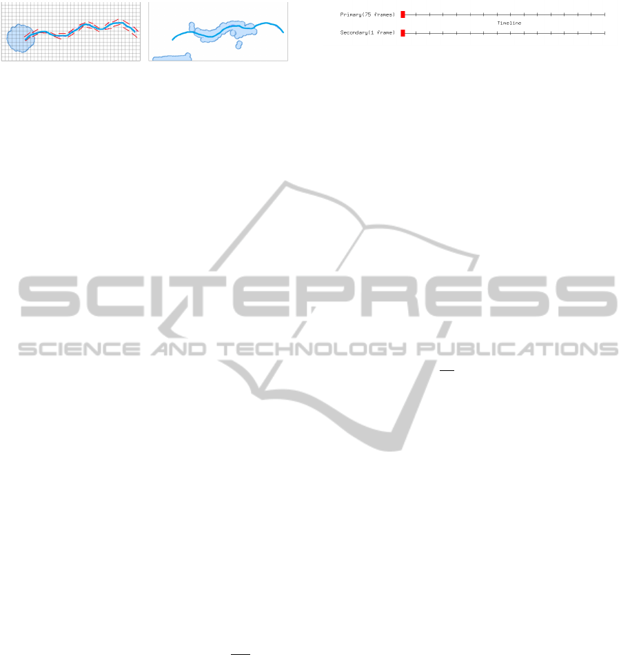
Figure 3: (a) shows a blob of fluid with the stroke. The
stroke alters the local velocity field around it. The velocity
vectors drawn in red are tangential to the smooth stroke.
The fluid flows in the altered velocity field as is shown in
(b).
3 STROKE-BASED INTERFACE
Strokes locally alter velocity field of fluid to create
desired fluid flows. The strokes are drawn as smooth
spline curves. These pass through the stroke points
that make up a mouse or pen gesture used to draw
the stroke. The grid cells through which the strokes
pass are identified. The horizontal and vertical com-
ponents of fluid velocity in these cells are modified
so that the resultant velocity matches the tangent to
the stroke at the point on the stroke that is closest to
the cell center. This process is illustrated in Figure 2.
The magnitude of the velocity can also be amplified
to match a strength value associated with each stroke.
Screenshots showing an example of this interaction in
our simulator are shown in Figure 3. Here a blob of
fluid is made to flow to the right by introducing a ve-
locity stroke.
Strokes not only put restriction on direction of
neighboring velocities but can also be used to control
their magnitude. Velocity strokes can be of different
strengths where their strength determines the magni-
tude of fluid velocity.
3.1 Timeline Control
The fluid simulation can only run at a timesteps at
which it satisfies the CourantFriedrichsLewy (CFL)
condition (Bridson, 2008) such that ∆t 6
∆x
v
max
. There
is however, a difference in the simulation timesteps
and the frame rate at which the animation is created.
Our interface maps the simulation time to correspond-
ing animation frames on a timeline. This timeline al-
lows the animator to paint the strokes at a particular
frame and have them active for a finite interval. Then
they can be deactivated. We have divided our timeline
in two parts (see Figure 4), primary and secondary.
The primary timeline has step size of 75 and the sec-
ondary timeline has step size of 1. This allows for fine
level keyframe control.
An example of this control can be seen in the re-
sult sequence shown in Figure 5. Here a blob of fluid
Figure 4: Primary and Secondary Timeline Controls.
splashes onto a fluid bed. The original simulation
shows only a small splash. The modified simulation
uses two different sets of strokes, active for different
time frames, to create a bigger splash.
4 ADDITIONAL CONTROLS
In addition to the stroke based control, we allow
for variable viscosity, arbitrarily shaped obstacles,
sources and sinks in our simulations.
4.1 Variable Viscosity
Viscosity is usually handled in fluid simulations by
implicitly solving a diffusion equation like
∂u
∂t
= ν∇
2
u (3)
In addition, solution of the Navier-Stokes introduces
numerical dissipation errors that visually appear as
viscosity in the simulation. In our simulator, we com-
pute fluid advection using a weighted combination
of the PIC and FLIP methods. This allows for vari-
able numerical dissipation. If even higher viscosities
are desired, the coefficient of viscosity, ν, is varied
and factored into the simulation by solving the diffu-
sion equation. This combination of viscosity inducing
methods is controlled by a single viscosity value. For
low viscous flows the viscosity value is less than 4
and only numerical viscosity is enough. Larger val-
ues of the viscosity values increase the coefficient of
viscosity.
Figure 6 shows a of frame of an animation at t = 2
seconds from the start of the animation where a blob
of fluid is splashing into a fluid bed. In 6(a) the fluid
has very low viscosity, so more fluid is displaced as
the blob hits the fluid bed and so the trough is deeper.
In 6(b) the trough is less deep for a more viscous fluid,
while in 6(c) the viscosity is so high that the fluid blob
is still falling down at this time frame.
4.2 Obstacles, Sources and Sinks
The animator can sketch arbitrary obstacles into the
simulation grid that can then interact with the grid.
Obstacles can be closed and open as shown in Fig-
ure 7. The simulator automatically sets appropriate
boundary conditions for these obstacles.
GRAPP2013-InternationalConferenceonComputerGraphicsTheoryandApplications
256
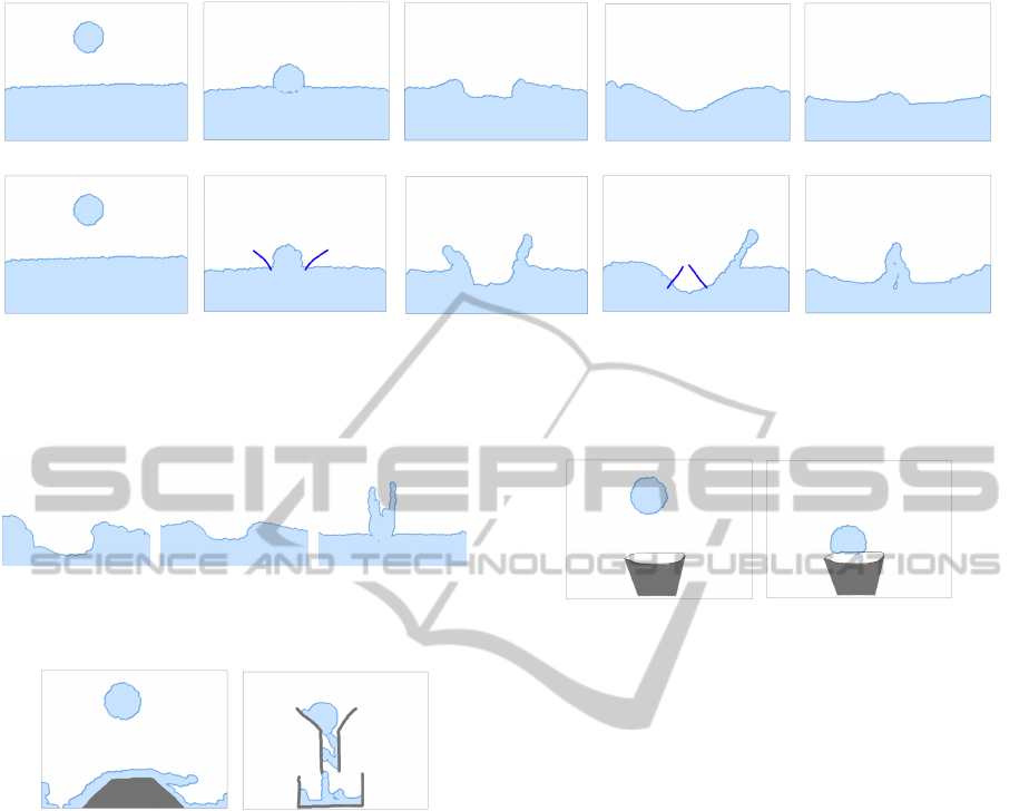
(a) (b) (c) (d) (e)
(f) (g) (h) (i) (j)
Figure 5: The top row shows the original simulation of a blob of fluid falling on a fluid bed. The bottom row shows two
strokes that are active only for finite time durations during the simulation that were used to modify the animation to create a
larger, more dramatic splash.
(a) (b) (c)
Figure 6: In (a) the viscosity value of the fluid is 1, in (b) it
is 5 and in (c) it is 10.
(a) (b)
Figure 7: (a) Shows a closed obstacle on which the fluid is
falling, (b) shows open obstacles used to model a funnel and
vessel with the fluid interacting with them.
The simulator can also handle various kinds of
fluid sources. Any arbitrary closed shape can be de-
fined to be a body of fluid by the animator. If the
shape is closed by the grid boundary on any side, it
is automatically detected and the grid boundary be-
comes the boundary for that source object (like the
fluid bed seen in Figure 5). Another type of source
that can be introduced are spherical blob sources of
various radii (an example of this is the drop of fluid
in Figure 5). These sources can introduce fluid into
the simulation at an artist specified rate, for an artist
specified time.
Similar to sources, arbitrary shapes sketched by
the artist can act as sinks. The boundary conditions
for sinks are adjusted automatically. Sinks can also
stay active for finite time durations if so desired by
the animator. Figure 8 shows a bucket shaped sink
sketched by the user. Figure 9 shows an arbitrary sink
(a) (b)
Figure 8: A bucket shaped sink absorbs the fluid blob that
falls into it.
absorbing fluid flying off a ramp shaped obstacle.
5 RENDERING
We experimented with many non-photorealistic ren-
dering techniques. Currently our rendering engine
support four kinds of renderers. For fast rendering we
use marker particles to track the fluid. The marker
particle positions are maintained in a dynamic ver-
tex buffer object which is used while rendering. The
first kind of rendering directly renders the points, as
shown in Figure 10(a). The next kind of renderer uses
point sprites, where a small texture is drawn at the
position of each marker particle and blended with the
neighbouring sprites using alpha blending, as shown
in Figure 10(b). The third kind of renderer uses a
modified marching squares algorithm to fill in the tri-
angles identified to get a solid filled fluid region (Fig-
ure 10(c)). Finally, we use a metaballs based renderer
that uses the metaball potential to color fluid region
(Figure 10(d)). The boundary metaballs are used to
draw a smooth boundary on the fluid surface. The
renderer can be swapped on the fly at runtime, as de-
sired by an artist.
In order to further enhance the shading, we have
modified the metaballs shader so that a gradient is
DirectableAnimationofNon-photorealisticFluids
257
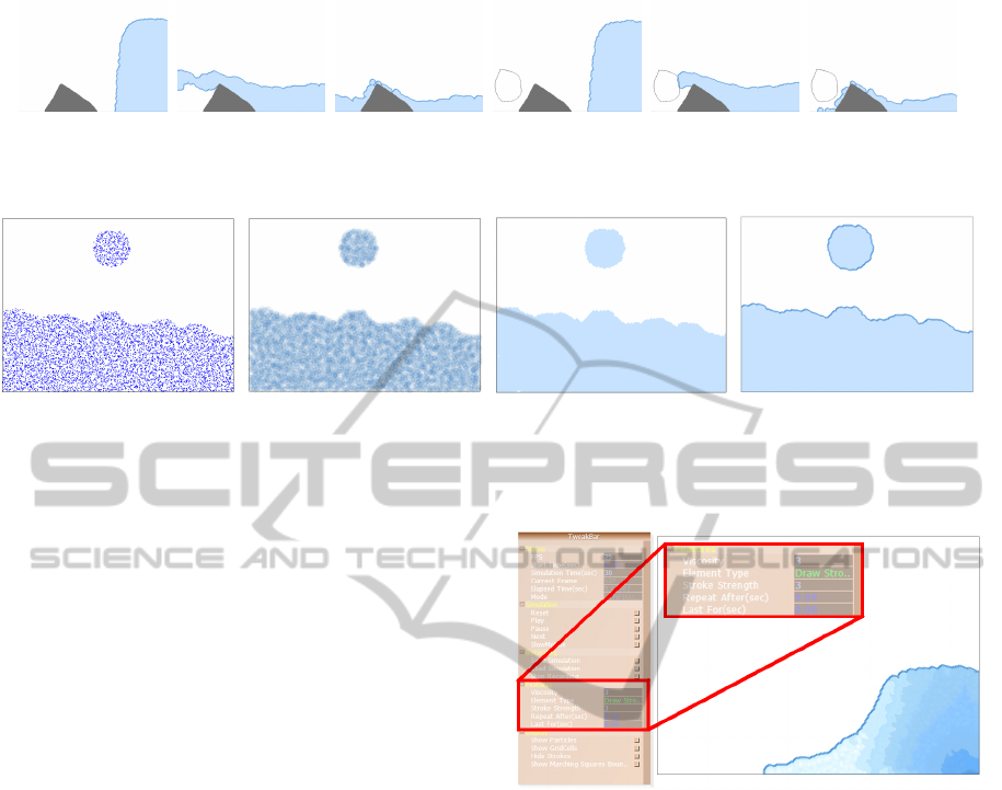
(a) (b) (c) (d) (e) (f)
Figure 9: (a), (b) and (c) show the original simulation of a blob of fluid flying of a ramp shaped obstacle. (d), (e) and (f) show
the fluid being absorbed by a sink sketched in by the artist.
(a) (b) (c) (d)
Figure 10: This image shows the various non-photorealistic renderers available in our simulator: (a) points, (b) point sprites,
(c) modified marching squares and (d) metaballs. For a 30 ×30 grid and 16 particles per grid cell, these methods take 2.33ms,
3.72ms, 4.33ms, 7.99ms respectively to render a frame of the simulation.
produced in the fluid mass based on the displacement
of the particles over a moving window of frames.
Thus, the color smoothly varies from light blue in fast
moving parts of the fluid to dark blue in slow moving
parts, as shown in Figures 1. The window ensures that
the color change is not abrupt in a particular region of
the fluid. Between different regions, the colors are
blended using the metaball potentials.
5.1 User Interface
The user interface consists of three main parts of
which the simulation area and the settings panel can
be seen in Figure 11, and a timeline control (see
Figure 4). A cropped, zoomed part of the settings
panel showing the controls available for strokes is also
shown. The panel allows animator to tune all con-
trol parameters like stroke strength, stroke duration,
source type, viscosity, obstacle type. The resulting
change in the simulation can be seen in realtime in
the simulation area. It also allows animator to add or
remove simulation elements to simulation area.
The timeline contains a slider which allows ani-
mator to move through frames. The artist can directly
draw on the simulation region to add strokes, obsta-
cles, sources or sinks. The simulation, once config-
ured, can also be recorded and played back.
6 TIMING RESULTS
We ran our simulator on a laptop machine with an ATI
Mobility Radeon HD 5470 graphics card, Intel core
Figure 11: The user interface.
i5-450M processor (3M cache, 2.40 GHz) and 4 GB
RAM. Then we timed a double dam-break experi-
ment, averaging the computation time spent for var-
ious sections of our simulator over 100 frames. The
results are shown in Tables 1(a) and 1(b).
Rendering time largely depends on the rendering
method used. Rendering using metaballs is computa-
tionally expensive and it takes the highest time (see
Figure 10. However, it can clearly be seen that even
on our modestly powered test laptop, the simulator
can easily work at 25 − 30 fps for the grid resolutions
reported. We have also tried our simulator on faster
machines where a much higher grid resolution can be
used with the simulator still working at realtime frame
rates.
7 CONCLUSIONS
We have presented an efficient and intuitive stroke-
based method for directing physically-based fluid
GRAPP2013-InternationalConferenceonComputerGraphicsTheoryandApplications
258
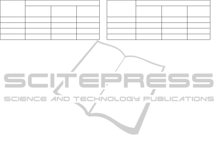
Table 1: (a) shows computation times for different grid resolutions with 16 particles per grid cell and a surface refinement
factor of 2. (b) shows computation times for different number of particles per grid for a grid resolution of 40 × 40 and surface
refinement factor of 1.
(a)
Grid Time (ms)
resolution Advection Projection Surface
Tracking
20 × 20 1.56 1.36 0.22
30 × 30 3.68 2.32 0.42
40 × 40 6.08 4.96 0.78
50 × 50 10.78 7.5 1.13
(b)
Particles Time (ms)
per grid cell Advection Projection Surface
Tracking
4 2.16 4.5 0.32
8 4.1 4.48 0.30
16 6.2 4.47 0.28
32 11.52 4.32 0.32
simulations in two-dimensions. The strokes can be
sketched by an artist on the simulation grid. They
automatically and locally alter the velocity field and
guide the fluid flow along their length. We also allow
the artist to sketch arbitrary shaped obstacles, sources
and sinks inside the simulation domain. All these el-
ements can be registered to a timeline easily, allow-
ing intuitive keyframing control to an animator. Fi-
nally, we allow for multiple non-photorealistic ren-
dering styles for the fluid. The simulator is efficient
enough to run at realtime rates and allows for all the
control to be done interactively.
We would like to extend our method to take ad-
vantage of stroke dynamics and layering of intersect-
ing strokes, which we cannot handle at present. Even
though we can handle variable viscosity in our sim-
ulator, we cannot simulate multi-phase flows. We
would like to extend this simulator to multi-phase
flows. Our current rendering mechanism does not
capture the specularity of fluids, which is frequently
used to make sketched fluids look better. We would
like our rendering method to be able to handle such
phenomena. We would also like to experiment more
with two-way solid-fluid coupling. Our current sim-
ulator already implements the variational framework
that can handle two-way coupling though we have not
experimented with it so far. Finally, we would like to
conduct an extensive user survey to gauge the efficacy
and intuitiveness of our interface for fluid control.
REFERENCES
Batty, C., Bertails, F., and Bridson, R. (2007). A fast vari-
ational framework for accurate solid-fluid coupling.
ACM Trans. on Graphics, 26(3):100.
Bergou, M., Mathur, S., Wardetzky, M., and Grinspun, E.
(2007). Tracks: toward directable thin shells. ACM
Trans. on Graphics, 26(3).
Blinn, J. F. (1982). A generalization of algebraic surface
drawing. ACM Trans. on Graphics, 1(3):235–256.
Bridson, R. (2008). Fluid Simulation For Computer Graph-
ics. A K Peters.
Chentanez, N., Goktekin, T. G., Feldman, B. E., and
O’Brien, J. F. (2006). Simultaneous coupling of fluids
and deformable bodies. In Proceedings of the SCA,
pages 83–89.
DeCarlo, D., Finkelstein, A., Rusinkiewicz, S., and San-
tella, A. (2003). Suggestive contours for conveying
shape. ACM Trans. on Graphics, 22(3):848–855.
Eden, A. M., Bargteil, A. W., Goktekin, T. G., Eisinger,
S. B., and O’Brien, J. F. (2007). A method for cartoon-
style rendering of liquid animations. In Proceedings
of Graphics Interface, pages 51–55. ACM.
Foster, N. and Fedkiw, R. (2001). Practical animation of
liquids. In Proceedings of SIGGRAPH, pages 23–30.
Foster, N. and Metaxas, D. (1996). Realistic animation
of liquids. Graphical Models and Image Processing,
58:471–483.
Foster, N. and Metaxas, D. (1997). Controlling fluid anima-
tion. In Proceedings of CGI.
Gilland, J. (2009). Elemental Magic , Volume 1: The Art of
Special Effects Animation. Focal Press.
Gooch, B. and Gooch, A. (2001). Non-Photorealistic Ren-
dering. AK Peters Ltd.
Gooch, B., Sloan, P.-P. J., Gooch, A., Shirley, P., and
Riesenfeld, R. (1999). Interactive technical illustra-
tion. In Proceedings of I3D, pages 31–38. ACM.
Lorensen, W. E. and Cline, H. E. (1987). Marching cubes:
A high resolution 3d surface construction algorithm.
Computer Graphics, SIGGRAPH 87, 21(4).
McNamara, A., Treuille, A., Popovi
´
c, Z., and Stam, J.
(2004). Fluid control using the adjoint method.
In ACM SIGGRAPH 2004 Papers, pages 449–456.
ACM.
Mihalef, V., Metaxas, D., and Sussman, M. (2004). Anima-
tion and control of breaking waves. In Proceedings of
the SCA, pages 315–324. Eurographics Association.
Rasmussen, N., Enright, D., Nguyen, D., Marino, S., Sum-
ner, N., Geiger, W., Hoon, S., and Fedkiw, R. (2004).
Directable photorealistic liquids. In Proceedings of
the SCA, pages 193–202. Eurographics Association.
Rost, R. and Kessenich, J. (2006). OpenGL Shading Lan-
guage. Addison-Wesley.
Shi, L. and Yu, Y. (2005). Controllable smoke animation
with guiding objects. ACM Transactions on Graphics,
24(1):140–164.
Stam, J. (1999). Stable fluids. In Proceedings of SIG-
GRAPH, pages 121–128.
DirectableAnimationofNon-photorealisticFluids
259

Thorne, M., Burke, D., and van de Panne, M. (2004). Mo-
tion doodles: an interface for sketching character mo-
tion. ACM Trans. on Graphics, 23(3).
Th
¨
urey, N., Keiser, R., Pauly, M., and R
¨
ude, U. (2006).
Detail-preserving fluid control. In Proceedings of the
SCA, pages 7–12. Eurographics Association.
Zhao, H. (2004). A fast sweeping method for Eikonal equa-
tions. Mathematics of Computation, 74(250):603–
627.
Zhu, B., Iwata, M., Haraguchi, R., Ashihara, T., Umetani,
N., Igarashi, T., and Nakazawa, K. (2011). Sketch-
based dynamic illustration of fluid systems. ACM
Trans. on Graphics, 30(6):134:1–134:8.
Zhu, Y. and Bridson, R. (2005). Animating sand as a fluid.
ACM Trans. on Graphics, 24:965–972.
GRAPP2013-InternationalConferenceonComputerGraphicsTheoryandApplications
260
