A Robust Least Squares Solution to the Relative Pose Problem on
Calibrated Cameras with Two Known Orientation Angles
Gaku Nakano and Jun Takada
Information and Media Processing Laboratories, NEC, Kawasaki, Japan
Keywords:
Two-view Geometry, Relative Pose Problem, Essential Matrix, Structure from Motion.
Abstract:
This paper proposes a robust least squares solution to the relative pose problem on calibrated cameras with
two known orientation angles based on a physically meaningful optimization. The problem is expressed as
a minimization problem of the smallest eigenvalue of a coefficient matrix, and is solved by using 3-point
correspondences in the minimal case and more than 4-point correspondences in the least squares case. To
obtain the minimum error, a new cost function based on the determinant of a matrix is proposed instead of
solving the eigenvalue problem. The new cost function is not only physically meaningful, but also common
in the minimal and the least squares case. Therefore, the proposed least squares solution is a true extension of
the minimal case solution. Experimental results of synthetic data show that the proposed solution is identical
to the conventional solutions in the minimal case and it is approximately 3 times more robust to noisy data
than the conventional solution in the least squares case.
1 INTRODUCTION
The relative pose problem on calibrated cameras is
to estimate an Euclidean transformation between two
cameras capturing the same scene from different po-
sitions. It is the most basic theory for an image based
3D reconstruction. ”Calibrated” means that the in-
trinsic camera parameters, e.g., the focal length, are
assumed to be known.
The general relative pose problem is expressed
by 5 parameters, i.e., 3 orientation angles and a 3D
translation vector up to scale. The absolute scale fac-
tor cannot be estimated without any prior knowledge
about the scene. One point correspondence gives one
constraint between the correspondence and the rela-
tive pose. The general relative pose problem is solved
by at least 5 point correspondences. Many solutions
based on point correspondences have been proposed,
which are called 5-point (Philip, 1996), (Triggs,
2000), (Nister, 2003), (Stew´enius et al., 2006), (Li
and Hartley, 2006), (Kukelova et al., 2008b), (Kalan-
tari et al., 2009b), 6-point (Pizarro et al., 2003),
7-point (Hartley and Zisserman, 2004) and 8-point
(Hartley and Zisserman, 2004) algorithm.
Meanwhile, a restricted relative pose problem
has been raised in which two orientation angles are
known. Two known orientation angles are obtained
by an IMU (internal measurement unit) sensor or a
vanishing point. Using the known angles brings two
great benefits. The one is that an angle measured by
high accurate sensors is more reliable than that ob-
tained by the point correspondencesbased algorithms.
The other is that the relative pose problem becomes
simpler since the degree of freedom is reduced to 3.
Therefore, the relative problem is solved by at least 3
point correspondences. It reduces the computational
cost of the pose estimation and also reduces the num-
ber of iterations of RANSAC (Fischler and Bolles,
1981).
Actual IMU sensors in many consumer products
do not have high accuracy needed in those solutions
due to noise caused by camera shake and tempera-
ture change. Therefore, pragmatic solutions to the re-
stricted pose problem must provide robustness to not
only image noise but also sensor noise.
Although some solutions are proposed for the re-
stricted problem, they are not robust and are not able
to estimate the optimal relative pose. A solution to the
3-point minimal case is first proposed in (Kalantari
et al., 2009a). The problem is formulated as a system
of multivariate polynomial equations, and is solved
by using a Gr¨obner basis method. Since the Gr¨obner
basis method requires a large computational cost to
decompose large matrices, Kalantari et al.’s solution
is not suitable for a RANSAC scheme. Fraundorfer et
al. propose 3 solutions (Fraundorfer et al., 2010). The
147
Nakano G. and Takada J..
A Robust Least Squares Solution to the Relative Pose Problem on Calibrated Cameras with Two Known Orientation Angles.
DOI: 10.5220/0004277801470154
In Proceedings of the International Conference on Computer Vision Theory and Applications (VISAPP-2013), pages 147-154
ISBN: 978-989-8565-48-8
Copyright
c
 2013 SCITEPRESS (Science and Technology Publications, Lda.)

Figure 1: the relative pose problem on calibrated cameras
with two known orientation angles.
one is to the minimal case, and the others are to the
least squares case of 4 and more than 5 point corre-
spondences. Fraundorfer et al. show that the minimal
solution is efficient for a RANSAC scheme. How-
ever, the two least squares solutions are not optimal
because they do not optimize a physically meaningful
cost function with 3 degrees of freedom.
This paper proposes a robust least squares solu-
tion to the relative pose problem on calibrated cam-
eras with two known orientation angles based on a
physically meaningful optimization. The problem is
formulated as a minimization problem of the small-
est eigenvalue of a coefficient matrix. To obtain the
minimum error, a new cost function based on the de-
terminant of a matrix is proposed instead of solving
the eigenvalue problem. The new cost function is not
only physically meaningful, but also common in the
minimal and the least squares case. Therefore, the
proposed least squares solution is a true extension of
the minimal case solution.
2 PROBLEM STATEMENT
This section describes the relative pose problem on
calibrated cameras with two known orientation an-
gles. Figure 1 shows an example of the problem such
that the two orientation angles are obtained by the
gravity direction g
g
g.
Let x
x
x and x
x
x
′
be point correspondences represented
by 3D homogeneouscoordinates in the image 1 and 2,
respectively. Then, the general relative pose problem
is written in the form
x
x
x
′T
[t
t
t]
×
R
R
R
z
R
R
R
y
R
R
R
x
x
x
x = 0. (1)
where t
t
t = [t
x
,t
y
,t
z
] denotes a 3D translation vector
up to scale, [ ]
×
denotes a 3× 3 skew symmetric ma-
trix representation of the vector cross product and R
R
R
x
,
R
R
R
y
and R
R
R
z
are 3 × 3 rotation matrices around x, y and
z-axis, respectively. Eq. (1) has 5 degrees of freedom
(2 degrees from t
t
t and 3 degrees from R
R
R
x
, R
R
R
y
and R
R
R
z
.)
Let φ, ψ and θ be the orientation angles around x,
y and z-axis, respectively. R
R
R
x
, R
R
R
y
and R
R
R
z
are expressed
as
R
R
R
x
=


1 0 0
0 cos(φ) sin(φ)
0 −sin(φ) cos(φ)


, (2)
R
R
R
y
=


cos(ψ) 0 sin(ψ)
0 1 0
−sin(ψ) 0 cos(ψ)


, (3)
R
R
R
z
=


cos(θ) sin(θ) 0
−sin(θ) cos(θ) 0
0 0 1


. (4)
If an IMU sensor is embedded in the cameras or
if a vanishing point is detected in the images, the two
orientation angles around x and y-axis, i.e., φ and ψ,
are known. Since R
R
R
x
and R
R
R
y
are given by Eqs. (2) and
(3), R
R
R
y
R
R
R
x
x
x
x can be simply expressed by x
x
x. Then, we
have
x
x
x
′T
[t
t
t]
×
R
R
R
z
x
x
x = 0. (5)
Equation (5) represents the relative pose problem
with two known orientation angles. The degree of
freedom of Eq. (5) is reduced to 5− 2 = 3.
Replacing [t
t
t]
×
R
R
R
z
by a 3× 3 matrix E
E
E, Eq. (5) can
be written in the linear form
x
x
x
′T
E
E
Ex
x
x = 0. (6)
Here, E
1,1
= E
2,2
, E
1,2
= −E
2,1
and E
3,3
= 0. E
i, j
is the element of E
E
E at the i–th row and the j–th col-
umn.
E
E
E is called the essential matrix if and only if the
two of its singular values are nonzero and equal, and
the third one is zero (Faugeras, 1993). These con-
straints are expressed by
det(E
E
E) = 0, (7)
E
E
EE
E
E
T
E
E
E −
1
2
trace(E
E
EE
E
E
T
)E
E
E = 0
3×3
. (8)
E
E
E has 6 parameters. However, the degree of free-
dom is 3 due to the scale ambiguity and the above
constraints (Fraundorfer et al., 2010).
Solving a nonlinear equation Eq. (5) and solving a
linear equation Eq. (6) with the nonlinear constraints
Eqs. (7) and (8) are identical.
VISAPP2013-InternationalConferenceonComputerVisionTheoryandApplications
148

3 PREVIOUS WORK
This section briefly describes about the conventional
solutions of (Kalantari et al., 2009a) and (Fraundorfer
et al., 2010), and points out the drawbacks of them.
The algorithm outlines of them are shown in Figures
2(a) and 2(b), respectively.
3.1 Kalantari et al.’s Solution
Kalantari et al. propose a solution to obtain all un-
knowns in Eq. (5) by solving a system of multivariate
polynomial equations.
Firstly, the Weierstrass substitution is used to ex-
press cos(θ) and sin(θ) without the trigonometric
functions: cos(θ) = (1 − p
2
)/(1 − p
2
) and sin(θ) =
2p/(1 + p
2
), where p = tan(θ/2). By substituting
3 point correspondences into Eq. (5) and by adding
a new scale constraint kt
t
tk = 1, there are 4 polyno-
mial equations in 4 unknowns {t
x
,t
y
,t
z
, p} of degree
3. Kalantari et al. adopt a Gr¨obner basis method to
solve the system of polynomial equations. The solu-
tions are obtained by Gauss-Jordan elimination of a
65× 77 Macaulay matrix and eigenvalue decomposi-
tion of a 12 × 12 Action matrix. Finally, at most 12
solutions are given from the eigenvectors.
Kalantari et al.’s solution takes much more com-
putational cost than the point correspondence based
algorithms due to decomposition of large matrices.
Moreover, it is difficult to extend to the least squares
case in which the degree of polynomial equations be-
comes higher and the size of matrices becomes a few
hundred dimensions.
In the experiment in this paper, the size of the de-
composed matrices and the number of the solutions
are not same as (Kalantari et al., 2009a). The details
of the implementation are described in section 5.2.
3.2 Fraundorfer et al.’s Solution
Fraundorfer et al. estimate the essential matrix in Eq.
(6) instead of the physical parameters. The most im-
portant contribution is to propose solutions to the least
squares case.
Fraundorfer et al. propose 3 solutions to the case
of 3 point, 4 point and more than 5 point correspon-
dences. The basic idea is very similar to the point
correspondences based algorithms, i.e., the 5-point,
the 7-point and the 8-point algorithm.
From a set of n point correspondences, Eq. (6) can
be equivalently written as
M
M
Mvec(E
E
E) = 0
n×1
, (9)
where M
M
M =

x
x
x
1
⊗ x
x
x
′
1
·· · x
x
x
n
⊗ x
x
x
′
n

T
and vec( )
denotes the vectorization of a matrix. ⊗ denotes the
Kronecker product.
The solution of Eq. (9) is obtained by
E
E
E =
6−n
∑
i=1
a
i
V
V
V
i
, (10)
where V
V
V
i
is the matrix corresponding to the gen-
erators of the right nullspace of the coefficient matrix
M
M
M, and a
i
is an unknown coefficient.
Estimating E
E
E is equivalent to calculate a
i
. One of
a
i
can be set to 1 to reduce the number of unknowns
due to the scale ambiguity of E
E
E. In the 3-point case,
Eqs. (7) and (8) are used to solve 2 unknowns. Sim-
ilarly, Eq. (7) is used to solve 1 unknown in the 4-
point case. For more than 5 point correspondences,
the solution is obtained by taking the eigenvector cor-
responding to the smallest eigenvalue of M
M
M
T
M
M
M.
An essential matrix can be decomposed to 2 R
R
R
z
s
and ±t
t
t (Horn, 1990), (Hartley and Zisserman, 2004).
Fraundorfer et al.’s 3-point, 4-point and 5-point algo-
rithm estimate at most 4, 3 and 1 essential matrices,
respectively. Therefore, they give at most 16, 12 and
4 solutions.
Fraundorfer et al.’s 3-point algorithm satisfies all
the constraints. However, the 4-point algorithm con-
siders only one constraint, and the 5-point algorithm
does not consider any constraints. For this reason, the
solutions of the 4-point and the 5-point algorithm may
not be an essential matrix. To correct an estimated
E
E
E to an essential matrix, a constraint enforcement is
carried out by replacing the singular values of E
E
E so
that the two are nonzero and equal, and the third one
is zero. The enforcement does not guarantee to opti-
mize θ and t
t
t which minimize Eq. (6) but the change
of the Frobenius norm. The 4-point and the 5-point al-
gorithm do not minimize physically meaningful cost
function, therefore, they are not optimal solution.
4 PROPOSED SOLUTION
This section describes about the basic idea of the pro-
posed solution in the minimal case firstly, and how to
extend the idea to the least squares case secondly. The
algorithm outline is shown in Figure 2(c).
4.1 3-point Algorithm for the Minimal
Case
Equation (5) can be equivalently written as
v
v
v
T
t
t
t = 0, (11)
ARobustLeastSquaresSolutiontotheRelativePoseProblemonCalibratedCameraswithTwoKnownOrientationAngles
149

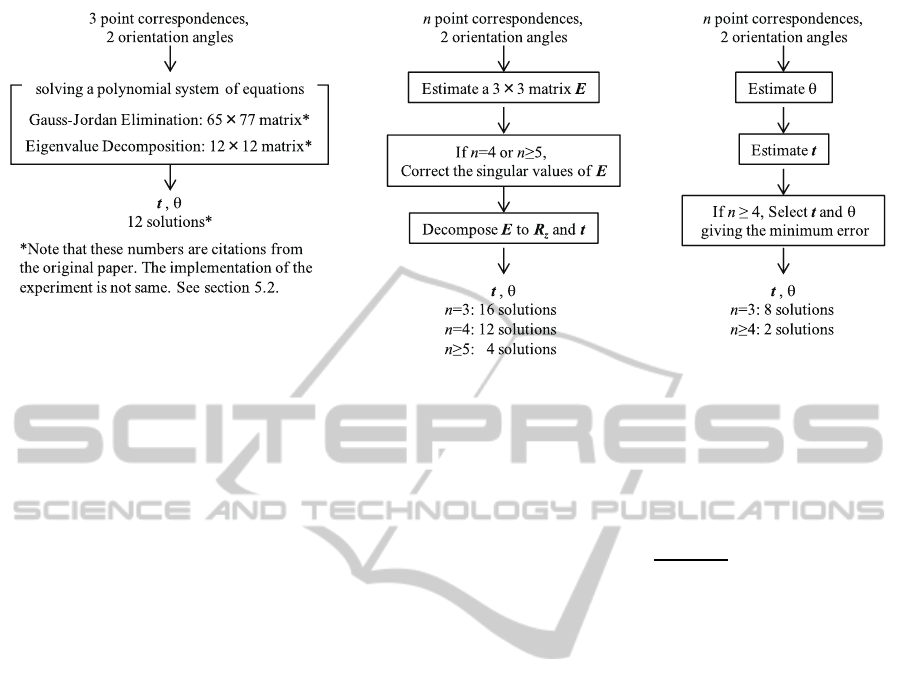
(a) Kalantari et al.’s Solution (b) Fraundorfer et al.’s Solution (c) Proposed Solution
Figure 2: Outlines of the conventional and the proposed solution.
where v
v
v = [x
x
x
′
]
T
×
R
R
R
z
x
x
x.
Given 3 point correspondences, we have
A
A
At
t
t = 0
3×1
, (12)
where A
A
A = [v
v
v
1
,v
v
v
2
,v
v
v
3
]
T
is a 3×3 coefficient matrix
involving the unknown θ.
Equation (12) shows that A
A
A is singular and t
t
t is
the nullspace of A
A
A. Therefore, θ is the solution of
det(A
A
A) = 0.
In the proposed 3-point algorithm, cos(θ) and
sin(θ) are replaced by new unknowns c and s, re-
spectively, instead of using the Weierstrass substitu-
tion. The reason is that it changes the range such that
−π ≤ θ ≤ +π to −∞ < p < +∞. This may cause com-
putational instability. Furthermore, a symbolic frac-
tional calculation makes polynomial equations com-
plex in the least squares case.
The unknowns c and s are obtained by solving the
following system of polynomial equations:
(
f
1
(c,s) = det(A
A
A) = 0,
g(c,s) = c
2
+ s
2
− 1 = 0.
(13)
Equation (13) can be solved by the resultant based
method which is also known as the hidden variable
method (Cox et al., 2005). Let f
1
and g be polynomial
equations of s, and c be regarded as a constant, the
resultant Res( f
1
,g,c) = 0 is a 4th degree univariate
polynomial in c. We get at most 4 solutions as the
real roots of Res( f
1
,g,c) = 0.
As a result, θ is obtained by
θ = atan2(s,c). (14)
Subsisting estimated θ into Eq. (12), t
t
t is obtained
by the cross product of two arbitrary rows of A
A
A. The
largest of these three cross products should be chosen
for numerical stability (Horn, 1990).
If v
v
v
i
× v
v
v
j
is the largest, we get t
t
t up to scale,
t
t
t = ±
v
v
v
i
× v
v
v
j
kv
v
v
i
× v
v
v
j
k
. (15)
The proposed 3-point algorithm gives at most 8
possible combinations of 4 θs and ±t
t
t.
4.2 4-point Algorithm for the Least
Squares Case
This section describes how to extend the proposed 3-
point algorithm to the least squares case.
Given more than 4 point correspondences, the
pose estimation problem is expressed by an optimiza-
tion problem:
minimize
t
t
t,θ
kB
B
Bt
t
tk
2
(16)
subject to kt
t
tk = 1
where B
B
B = [v
v
v
1
,· ·· ,v
v
v
n
]
T
is an n× 3 coefficient ma-
trix involving the unknown θ, and kt
t
tk = 1 is a con-
straint to avoid the trivial solution t
t
t = 0
3×1
.
As widely known in the 8-point algorithm, the op-
timal t
t
t is the eigenvector corresponding to the small-
est eigenvalue of B
B
B
T
B
B
B and the minimum error of the
cost function kB
B
Bt
t
tk
2
is equal to the smallest eigenvalue
of B
B
B
T
B
B
B. The optimization problem Eq. (16) is essen-
tially identical to the eigenvalue problem. However, it
is difficult to compute directly the smallest eigenvalue
of B
B
B
T
B
B
B represented by a complex number.
To avoid the eigenvalue computation, this paper
proposesa new cost function, det(B
B
B
T
B
B
B). The determi-
nant is equal to the product of all eigenvalues and B
B
B
T
B
B
B
VISAPP2013-InternationalConferenceonComputerVisionTheoryandApplications
150

is positive semidefinite. Therefore, kB
B
Bt
t
tk
2
is assumed
to be minimized if det(B
B
B
T
B
B
B) is minimized. Thus, the
proposed 4-point algorithm minimizes det(B
B
B
T
B
B
B) in-
stead of kB
B
Bt
t
tk
2
.
Similar to the proposed 3-point algorithm, θ is ob-
tained by solving the following polynomial system of
equations:





f
2
(c,s) =
d
dθ
det(B
B
B
T
B
B
B)



cos(θ)=c,
sin(θ)=s
= 0,
g(c,s) = c
2
+ s
2
− 1 = 0.
(17)
Here,
d
dθ
det(B
B
B
T
B
B
B)



cos(θ)=c,
sin(θ)=s
denotes that cos(θ) and
sin(θ) in
d
dθ
det(B
B
B
T
B
B
B) are replaced by c and s, respec-
tively.
The resultant Res( f
2
,g,c) = 0 is an 8th degree
univariate polynomial in c. We get the optimal θ from
the real roots so that it minimizes det(B
B
B
T
B
B
B) or the
eigenvalue of B
B
B
T
B
B
B.
Finally, we obtain the optimal t
t
t by taking the
eigenvector corresponding to the smallest eigenvalue
of B
B
B
T
B
B
B. The proposed4-point algorithm gives at most
2 possible combination of one θ and ±t
t
t.
Moreover, the proposed 4-point algorithm in-
cludes the solutions of the proposed 3-point algo-
rithm. For this reason, the proposed 4-point algorithm
is a true extension of the 3-point algorithm. The proof
is described in Appendix.
5 EXPERIMENTS
5.1 Synthetic Data
The robustness of the proposed solutions are evalu-
ated under various image and angle noise. 3D points
are generated randomly similar to (Fraundorfer et al.,
2010) so that the 3D points have a depth of 50% of the
distance of the first camera to the scene. In (Fraun-
dorfer et al., 2010), 2 camera configurations are per-
formed, i.e., sideway and forward motion with ran-
dom rotation. To simulate more realistic environment,
random motion with random rotation is performed in
this experiment. The baseline between the two cam-
eras is 10% of the distance to the scene.
Kalantari et al. and Fraundorfer et al. assume
that the error of the two orientation angles measured
by a low cost sensor is from 0.5 [degree] to at most
1.0 [degree]. However, the accuracy of almost of all
low cost sensors are not necessarily opened. Some of
them may have more larger noise than 1.0 [degree].
Therefore, in this experiment, the error is assumed at
most 3.0 [degree].
For an image noise test, the standard deviation of
Gaussian noise is fixed σ = 0.5 [degree] for the two
known angles, and is changed 0≤ σ ≤ 3 [pixel] for the
point correspondences. Similarly, for an angle noise
test, the standard deviation is fixed σ = 0.5 [pixel] for
the point correspondences, and is changed 0 ≤ σ ≤ 3
[degree] for the two known angles.
The estimation errors of θ and t
t
t are evaluated as
follows:
Error(θ
est
,θ
true
) = abs(θ
est
− θ
true
), (18)
Error(t
t
t
est
,t
t
t
true
) = cos
−1

t
t
t
T
est
t
t
t
true
kt
t
t
est
kkt
t
t
true
k

, (19)
where the subscript est and true denote the es-
timated and the ground truth value, respectively. If
multiple solutions are found, the one having mini-
mum error is selected. The RMS (root mean square)
errors in degrees are plotted over 500 independent tri-
als for each noise level in the result figures.
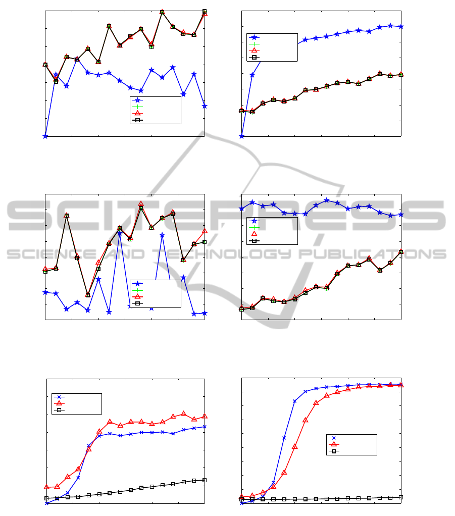
5.2 Results of the Minimal Case
The robustness of the proposed are evaluated in the
minimal case and compared to the two conventional
3-point algorithms and Nister’s 5-point algorithm
based on point correspondences. The conventional 3-
point algorithms are implemented by the authors and
the 5-point algorithm is implemented by H. Stewe-
nius
1
. Kalantari et al’s solution is implemented by
using Kukelova’s automatic generator of Gr¨obner ba-
sis solvers (Kukelova et al., 2008a)
2
. As mentioned in
section 3.1, the matrix sizes are not same as the orig-
inal. The Macaulay matrix is 58 × 66 and the Action
matrix is 8× 8 in this experiment.
As shown in Figures 3 and 4, all the 3-point al-
gorithms are almost same performance. There is no
difference between the degree of freedom of each al-
gorithm. Thus, all the 3-point algorithms solve the
mathematically identical problem.
5.3 Results of the Least Squares Case
The robustness of the proposed 4-point algorithm are
evaluated in the least squares case and compared to
Fraundorfer et al.’s 5-point algorithm and Hartley’s 8-
point algorithm based on point correspondences. All
algorithms are implemented by the authors.
Figure 5 shows the robustness for 100 point cor-
respondences with the fixed angle noise and variable
1
http://www.vis.uky.edu/∼stewe/FIVEPOINT/
2
http://cmp.felk.cvut.cz/minimal/automatic generator.php
ARobustLeastSquaresSolutiontotheRelativePoseProblemonCalibratedCameraswithTwoKnownOrientationAngles
151

0 0.5 1 1.5 2 2.5 3
0
2
4
6
8
10
12
14
RMS Rotation Error (Random Motion)
Gaussian Image Noise [pixels]
Rotation Error [degree]
Nister 5pt
Kalantari 3pt
Fraundorfer 3pt
Proposed 3pt
(a) RMS error of θ
0 0.5 1 1.5 2 2.5 3
0
10
20
30
40
50
60
70
80
RMS Translation Error (Random Motion)
Gaussian Image Noise [pixels]
Translation Error [degree]
Nister 5pt
Kalantari 3pt
Fraundorfer 3pt
Proposed 3pt
(b) RMS error of t
t
t
Figure 3: Results of the minimal case with fixed angle noise and variable image noise.
0 0.5 1 1.5 2 2.5 3
4
5
6
7
8
9
10
11
12
RMS Rotation Error (Random Motion)
Gaussian Angle Noise [degree]
Rotation Error [degree]
Nister 5pt
Kalantari 3pt
Fraundorfer 3pt
Proposed 3pt
(a) RMS error of θ
0 0.5 1 1.5 2 2.5 3
15
20
25
30
35
40
45
50
55
RMS Translation Error (Random Motion)
Gaussian Angle Noise [degree]
Translation Error [degree]
Nister 5pt
Kalantari 3pt
Fraundorfer 3pt
Proposed 3pt
(b) RMS error of t
t
t
Figure 4: Results of the minimal case with fixed image noise and variable angle noise.
0 0.5 1 1.5 2 2.5 3
0
0.2
0.4
0.6
0.8
1
1.2
1.4
RMS Rotation Error (Random Motion)
Gaussian Image Noise [pixels]
Rotation Error [degree]
Hartley 8pt
Fraundorfer 5pt
Proposed 4pt
(a) RMS error of θ
0 0.5 1 1.5 2 2.5 3
0
10
20
30
40
50
60
70
80
90
RMS Translation Error (Random Motion)
Gaussian Image Noise [pixels]
Translation Error [degree]
Hartley 8pt
Fraundorfer 5pt
Proposed 4pt
(b) RMS error of t
t
t
Figure 5: Results of the least squares case with fixed angle noise and variable image noise.
image noise. As the image noise becomes larger, the
error of the conventional algorithms become larger
sharply. By contrast, that of the proposed 4-point al-
gorithm is much less than them.
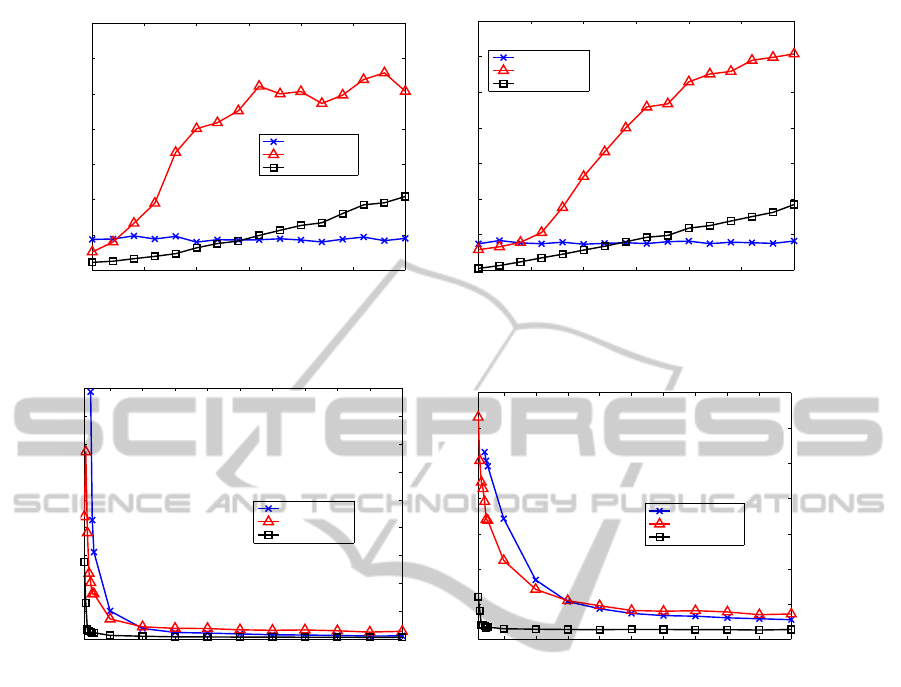
Figure 6 shows the result of the fixed image noise
and variable angle noise. Hartley’s 8-point algorithm
is not influenced by the angle noise because it does
not use the known angles. Fraundorfer et al.’s 5-point
algorithm is more accurate than Hartley’s 8-point al-
gorithm if the angle noise is less than 0.4 [degree].
The tolerance of the proposed 4-point algorithm is ap-
proximately 1.4 [degree]. This is 3 times more robust
than Fraundorfer et al.’s 5-point algorithm.
VISAPP2013-InternationalConferenceonComputerVisionTheoryandApplications
152

0 0.5 1 1.5 2 2.5 3
0
0.2
0.4
0.6
0.8
1
1.2
1.4
RMS Rotation Error (Random Motion)
Gaussian Angle Noise [degree]
Rotation Error [degree]
Hartley 8pt
Fraundorfer 5pt
Proposed 4pt
(a) RMS error of θ
0 0.5 1 1.5 2 2.5 3
0
10
20
30
40
50
60
70
RMS Translation Error (Random Motion)
Gaussian Angle Noise [degree]
Translation Error [degree]
Hartley 8pt
Fraundorfer 5pt
Proposed 4pt
(b) RMS error of t
t
t
Figure 6: Results of the least squares case with fixed image noise and variable angle noise.
20 40 60 80 100 120 140 160 180 200
0
1
2
3
4
5
6
7
8
9
RMS Rotation Error (Random Motion)
the Number of Point Correspondences
Rotation Error [degree]
Hartley 8pt
Fraundorfer 5pt
Proposed 4pt
(a) RMS error of θ
20 40 60 80 100 120 140 160 180 200
0
10
20
30
40
50
60
70
RMS Translation Error (Random Motion)
the Number of Point Correspondences
Translation Error [degree]
Hartley 8pt
Fraundorfer 5pt
Proposed 4pt
(b) RMS error of t
t
t
Figure 7: Results of changing the number of the point correspondences.
5.4 Results of Changing the Number of
the Point Correspondences
The influence of changing the number of the point
correspondences are evaluated in the least squares
case. The image and angle noise are fixed 0.5 [pixel]
and 0.5 [degree], respectively. From 4 to 200 point
correspondences are evaluated.
As shown in Figure 7, the proposed 4-point algo-
rithm is always best. It is notable that the proposed
4-point algorithm reaches the performance boundary
at 40–60 point correspondences, whereas the conven-
tional algorithms needs more than 100 point corre-
spondences. This is very important for practical use
since few dozens of point correspondences are ob-
tained generally. Moreover, for more than 40 point
correspondences, Fraundorfer et al.’s 5-point algo-
rithm is worse than Hartley’s 8-point algorithm which
uses only point correspondences. The proposed 4-
point algorithm outperforms both algorithm regard-
less of the number of the point correspondences.
According to the results in sections 5.2 and 5.3,
sufficiently robust and accurate solutions can be ob-
tained by the proposed cost function without solving
the eigenvalue problem.
6 CONCLUSIONS
A robust least squares solution to the relative pose
problem on calibrated cameras with two known orien-
tation angles are proposed in this paper. The problem
is expressed as a minimization problem of the small-
est eigenvalue of a coefficient matrix. To obtain the
minimum error, a new cost function based on the de-
terminant of a matrix is proposed instead of solving
the eigenvalue problem. The new cost function is not
only physically meaningful, but also common in the
minimal and the least squares case. The conventional
solutions employ different algorithms for the minimal
case and the least squares case. By contrast, the pro-
posed least squares solution is a true extension of the
minimal case solution. Experimental results of syn-
thetic data show that the proposed solution is identi-
ARobustLeastSquaresSolutiontotheRelativePoseProblemonCalibratedCameraswithTwoKnownOrientationAngles
153

cal to the conventional solutions in the minimal case
and it is approximately 3 times more robust to noisy
data than the conventionalsolution in the least squares
case. A real data experiment using consumer IMU
sensors is in the future research.
REFERENCES
Cox, D., Little, J., and O’Shea, D. (2005). Using Algebraic
Geometry. Springer, 2nd edition.
Faugeras, O. (1993). Three-dimensional computer vision: a
geometric viewpoint. the MIT Press.
Fischler, M. A. and Bolles, R. C. (1981). Random sample
consensus: a paradigm for model fitting with appli-
cations to image analysis and automated cartography.
Commun. ACM, 24(6):381–395.
Fraundorfer, F., Tanskanen, P., and Pollefeys, M. (2010). A
minimal case solution to the calibrated relative pose
problem for the case of two known orientation angles.
Computer Vision–ECCV 2010, pages 269–282.
Hartley, R. I. and Zisserman, A. (2004). Multiple View Ge-
ometry in Computer Vision. Cambridge University
Press, ISBN: 0521540518, second edition.
Horn, B. (1990). Recovering baseline and orientation from
essential matrix. J. Optical Society of America.
Kalantari, M., Hashemi, A., Jung, F., and Gu´edon, J.-P.
(2009a). A new solution to the relative orientation
problem using only 3 points and the vertical direction.
CoRR, abs/0905.3964.
Kalantari, M., Jung, F., Guedon, J., and Paparoditis, N.
(2009b). The five points pose problem: A new and
accurate solution adapted to any geometric configura-
tion. Advances in Image and Video Technology, pages
215–226.
Kukelova, Z., Bujnak, M., and Pajdla, T. (2008a). Auto-
matic generator of minimal problem solvers. Com-
puter Vision–ECCV 2008, pages 302–315.
Kukelova, Z., Bujnak, M., and Pajdla, T. (2008b). Polyno-
mial eigenvalue solutions to the 5-pt and 6-pt relative
pose problems. BMVC 2008, 2(5).
Li, H. and Hartley, R. (2006). Five-point motion estimation
made easy. In Pattern Recognition, 2006. ICPR 2006.
18th International Conference on, volume 1, pages
630–633. IEEE.
Nister, D. (2003). An efficient solution to the five-point rel-
ative pose problem. In Computer Vision and Pattern
Recognition, 2003. Proceedings. 2003 IEEE Com-
puter Society Conference on, volume 2, pages II–195.
IEEE.
Philip, J. (1996). A non-iterative algorithm for determining
all essential matrices corresponding to five point pairs.
The Photogrammetric Record, 15(88):589–599.
Pizarro, O., Eustice, R., and Singh, H. (2003). Relative
pose estimation for instrumented, calibrated imaging
platforms. Proceedings of Digital Image Computing
Techniques and Applications, Sydney, Australia, pages
601–612.
Stew´enius, H., Engels, C., and Nist´er, D. (2006). Re-
cent developments on direct relative orientation. IS-
PRS Journal of Photogrammetry and Remote Sensing,
60(4):284–294.
Triggs, B. (2000). Routines for relative pose of two cali-
brated cameras from 5 points. Technical Report, IN-
RIA.
APPENDIX
The proof of that the proposed 4-point algorithm in-
cludes the 3-point algorithm is as follows.
Substituting 3 point correspondences into Eq.
(17), we have
d
dθ
det(B
B
B
T
B
B
B) =
d
dθ
det(A
A
A
T
A
A
A)
=
d
dθ
det(A
A
A)
2
= 2det(A
A
A)
d
dθ
det(A
A
A).
(20)
We can construct a system of polynomial equa-
tions as follows:





f
3
(c,s) = det(A
A
A)
d
dθ
det(A
A
A)



cos(θ)=c,
sin(θ)=s
= 0,
g(c,s) = c
2
+ s
2
− 1 = 0.
(21)
The solutions of the resultant Res( f
3
,g,c) = 0 in-
cludes that of Res( f
1
,g,c) = 0.
VISAPP2013-InternationalConferenceonComputerVisionTheoryandApplications
154