Continuous Tracking of Structures from an Image Sequence
Yann Lepoittevin
1,2
, Dominique B
´
er
´
eziat
3
, Isabelle Herlin
1,2
and Nicolas Mercier
1,2
1
Inria, B.P. 105, 78153 Le Chesnay, France
2
CEREA, Joint Laboratory ENPC - EDF R&D, Universit
´
e Paris-Est,
Cit
´
e Descartes Champs-sur-Marne, 77455 Marne la Vall
´
ee Cedex 2, France
3
Universit
´
e Pierre et Marie Curie, 4 place Jussieu, Paris 750005, France
Keywords:
Tracking, Motion, Data Assimilation, Satellite image, Meteorology.
Abstract:
The paper describes an innovative approach to estimate velocity on an image sequence and simultaneously
segment and track a given structure. It relies on the underlying dynamics’ equations of the studied physical
system. A data assimilation method is applied to solve evolution equations of image brightness, those of
motion’s dynamics, and those of distance map modelling the tracked structures. Results are first quantified
on synthetic data with comparison to ground-truth. Then, the method is applied on meteorological satellite
acquisitions of a tropical cloud, in order to track this structure on the sequence. The outputs of the approach
are the continuous estimation of both motion and structure’s boundary. The main advantage is that the method
only relies on image data and on a rough segmentation of the structure at initial date.
1 INTRODUCTION
The issue of detecting and tracking a structure covers
a broad of major computer vision problems. Read-
ers can refer to (Yilmaz et al., 2006), for instance,
in order to get an extensive description on this issue.
However, images may be noisy, as this is the case for
satellite acquisitions, and assumptions on dynamics
should then be involved. To our knowledge, no paper
concerns a method that simultaneously estimates mo-
tion and segments/tracks a structure from only image
data and a rough segmentation of the structure. How-
ever, methods exist that segment and track a structure,
given motion field and initial segmentation (Peterfre-
und, 1999; Rathi et al., 2007; Avenel et al., 2009), or
that track a structure and estimate its motion if this
structure has been accurately segmented on the first
image (Bertalm
´
ıo et al., 2000).
The use of data assimilation recently emerged in
the image processing community. In (B
´
er
´
eziat and
Herlin, 2011), motion estimation is discussed, and
solutions are described for processing noisy images.
In (Papadakis and M
´
emin, 2008), an incremental 4D-
Var is used, that also computes motion field and tracks
a structure, but relies, as inputs, on both image data
and accurate segmentation of the structure on the
whole sequence. Our approach has the advantage to
simultaneously solve the issues of motion estimation,
detection, segmentation and tracking of the structure,
based, as only inputs, on image data and their gradient
values.
Section 2 describes the main mathematical com-
ponents of the approach. Sections 3 and 4 discuss
results obtained on synthetic data and meteorological
satellite acquisitions. Section 5 concludes with some
remarks and perspectives on the research work.
2 MATHEMATICAL SETTING
Our approach is based on a 4D-Var data assimilation
algorithm, used to estimate motion on the sequence
and track a structure.
Ω denotes the bounded image domain, on which
pixels x =

x y

T
are considered, [0, T ] the studied
temporal interval, and A = Ω × [0, T ].
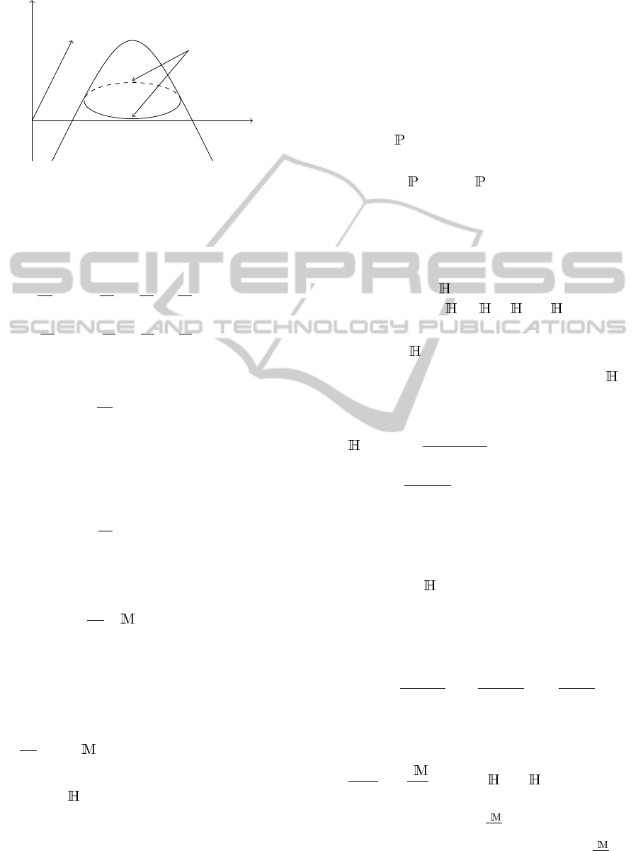
2.1 Model of Structure and Input Data
Let define the structure tracked along the image se-
quence by an implicit function φ (see Figure 1): each
pixel x at date t gets for value its signed distance to
the current position of the structure boundary.
Observations, used during the assimilation, are
images themselves and their contour points, obtained
by thresholding the maxima of the gradient norm.
386
Lepoittevin Y., Béréziat D., Herlin I. and Mercier N..
Continuous Tracking of Structures from an Image Sequence.
DOI: 10.5220/0004278503860389
In Proceedings of the International Conference on Computer Vision Theory and Applications (VISAPP-2013), pages 386-389
ISBN: 978-989-8565-48-8
Copyright
c
 2013 SCITEPRESS (Science and Technology Publications, Lda.)

x
φ(x, y)
y
φ(x, y) = 0
Figure 1: Implicit representation of structure’s boundary.
2.2 Evolution Model
The assumption on dynamics is the Lagrangian con-
stancy of velocity w =

u v

T
, rewritten as:
du
dt
= 0 ⇔
∂u
∂t
+ u
∂u
∂x
+ v
∂u
∂y
= 0 (1)
dv
dt
= 0 ⇔
∂v
∂t
+ u
∂v
∂x
+ v
∂v
∂y
= 0 (2)
A pseudo-image I
s
is defined, that satisfies the op-
tical flow constraint:
∂I
s
∂t
+ ∇I
s
.w = 0 (3)
The pseudo-image is compared to satellite data dur-
ing the optimization process: they have to be almost
identical at acquisition dates. The implicit function φ
is assumed to satisfy the same heuristics, as the struc-
ture moves accordingly to image evolution:
∂φ
∂t
+ ∇φ.w = 0 (4)
The state vector, defined as X =

u v I
s
φ

T
,
satisfies the evolution system (1, 2, 3, 4), summarized
by:
∂X
∂t
+ (X(t)) = 0 (5)
2.3 4D-Var Data Assimilation
In order to estimate X, and obtain motion estimation
and tracking of the structure, the 4D-Var algorithm
considers the following three equations:
∂X
∂t
(x, t) + (X)(x, t) = 0 (6)
X(x, 0) = X
b
(x) + ε
b
(x) (7)
(X, Y)(x, t) = ε
R
(x, t) (8)
The first one is the evolution equation. One can
notice that X(x, t), for any t, is determined from
X(x, 0) and the integration of Equation (6).
Equation (7) corresponds to the knowledge, that is
available on the state vector at initial date 0, and ex-
pressed as the background value X
b
(x). The solution
X(x, 0), estimated by 4D-Var, should stay close to this
background value. However, as it is uncertain, an er-
ror term, ε
b
(x), is considered. No knowledge is avail-
able on the initial velocity field and its background
value is null; the background on the pseudo-image I
s
is the first image of the sequence; and the background
of φ, denoted φ
b
, roughly defines the structure to be
tracked. Let be the projection of the state vector on
components I
s
and φ, Equation (7) is rewritten as:
(X(0)) = (X
b
) + ε
b
(9)
Equation (8), named observation equation, links
the observations to the state vector X. The obser-
vation vector Y includes the image acquisitions and
a distance map to the contour points, that have been
computed on these acquisitions. This distance map is
denoted by D
c
(x, t). denotes the observation opera-
tor, split in two parts: =

I φ

T
.
I
compares
pseudo-images I
s
to image observations I:
I
(X, Y) = I
s
− I = ε
I
(10)
Their discrepancy is described by the error ε
I
.
φ
compares φ to the distance map D
c
(x, t). The absolute
value of φ should be almost equal to D
c
:
φ
(X, Y) =
4e
−aφ
(1 + e
−aφ
)
2
(|φ| − D
c
) = ε
φ
(11)
The function
4e
−aφ
(1+e
−aφ
)
2
is introduced to decrease the
impact of contours, that do not belong to the bound-
ary of the tracked structure. Parameter a controls the
slope of the function. The more a increases, the more
the function looks like an indicator function: only pix-
els in a small neighborhood of structure’s boundary
are considered by
φ
during the optimization process.
Errors ε
b
, ε
I
, ε
φ
are supposed Gaussian, zero-
mean, not correlated, with respective variance B, R
I
,
R
φ
. Solving System (6, 9, 10, 11) is then written as
the minimization of the following cost function:
J(X(0)) =
Z
A
ε
I
(x, t)
2
R
I
(x, t)
+
Z
A
ε
φ
(x, t)
2
R
φ
(x, t)
+
Z
Ω
ε
b
(x)
2
B(x)
(12)
Let λ denote the adjoint variable, verifying:
λ(T ) = 0 (13)
−
∂λ(t)
∂t
+

∂
∂X

∗
λ(t) =
∗
R
−1
(X, Y)(t) (14)
with the adjoint operator

∂
∂X

∗
, which is defined
by:
h
Zη, λ
i
=
h
η, Z
∗
λ
i
. The adjoint operator

∂
∂X

∗
ContinuousTrackingofStructuresfromanImageSequence
387

is automatically generated from the discrete opera-
tor by an efficient automatic differentiation soft-
ware (Hasco
¨
et and Pascual, 2004). Then, gradient of
J is:
∂J
∂X(0)
=
T
B
−1
[ (X(0)) − (X
b
)] + λ(0) (15)
Minimization is achieved by a steepest method and
the L-BFGS algorithm (Zhu et al., 1997).
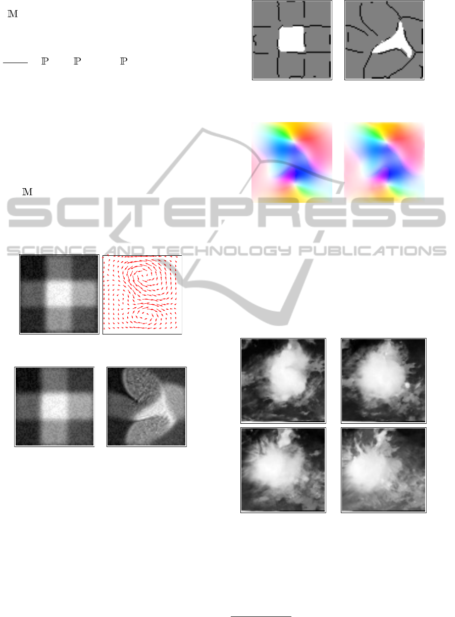
3 TWIN EXPERIMENT
A sequence of five Image Observations (see Figure 3),
I
i
= I(t
i
) for i = 1 to 5, is generated by integrating
model from initial conditions, displayed in Fig-
ure 2. Contours are first computed on images I
i
. Then
Distance Map Observations D
c
(x, t
i
) are derived. This
is done in order to estimate motion on the whole im-
age sequence and track the brightest square.
Figure 2: Left : initial image. Right : initial motion field.
Figure 3: Image Observations at t
1
and t
5
.
After assimilation, pseudo-images are compared
to Image Observations. They are almost identical and
their correlation measure is over 0.999. At dates t
i
,
the region of positive values of φ, corresponding to
the inside of the tracked structure, is compared to the
contour points, see Figure 4.
The simulation, that provides Image Observa-
tions, also provides ground-truth of the velocity field.
This allows to perform statistics on the discrepancy
between estimated motion and ground-truth: average
error is around 1% in norm and less than one degree
in orientation. Motion estimated on the whole image
is displayed on Figure 5 with the coloured representa-
Figure 4: Comparison of φ and contour points on Image
Observation. Left: t
1
, Right: t
5
.
Figure 5: Left: Ground-truth. Right: Assimilation result.
tion tool of the Middlebury database
1
: there is no vis-
ible difference between estimation and ground-truth.
4 METEOSAT IMAGES
The assimilation method is applied on a Meteosat se-
quence and displayed on Figure 6.
Figure 6: Images of a tropical cloud in the infrared domain.
From left to right, up to down.
Figure 7, first column, displays the contour points,
used to calculate the Distance Map Observations
D
c
(x, t
i
). Pseudo-images, obtained as result of data
assimilation, are displayed on the second column. On
the third column, the blue curve corresponds to the
1
http://vision.middlebury.edu/flow/
VISAPP2013-InternationalConferenceonComputerVisionTheoryandApplications
388

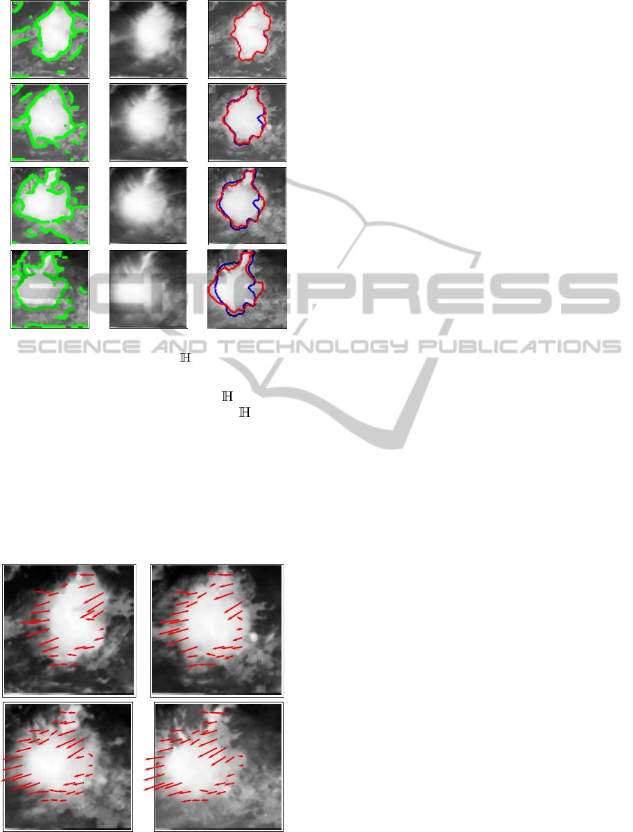
Figure 7: Left: Contours on observations. Middle: pseudo-
images. Right: red is the result with
φ
, blue is without.
result of assimilation without the term
φ
in Equa-
tion 11, while the red one is obtained with
φ
. As it
can be seen, including constraints on φ allows to im-
prove the accuracy of segmentation. Motion field is
estimated on the whole image, but Figure 8 focuses
on the boundary of the structure. It shows that the re-
sulting velocity vectors correctly assess displacement
of the structure along the sequence. The displacement
estimated at the boundary of the tracked structure, su-
perposed on satellite images, is shown on Figure 8.
Figure 8: Motion result superposed to images on the bound-
ary of the tracked structure. From left to right, up to down.
5 CONCLUSIONS
The paper describes an innovative approach enabling
to estimate motion, segment and track a structure on
images, such as, for instance, a cloud on a satellite se-
quence. The approach is based on 4D-Var data assim-
ilation, and the state vector includes an implicit func-
tion φ modelling the boundary of the tracked struc-
ture. Results are given on synthetic and meteoro-
logical data. Additional experiments have been con-
ducted, not described in the paper, that confirm the
robustness of the approach.
The main perspective of this research is to ex-
tend the method to multi-structures tracking and to
a space-time segmentation process. An additional in-
teresting perspective is to allow uncertainty on the dy-
namic equations and take into account a model error
in Equation (6).
REFERENCES
Avenel, C., M
´
emin, E., and P
´
erez, P. (2009). Tracking
closed curves with non-linear stochastic filters. In
Conference on Space-Scale and Variational Methods.
B
´
er
´
eziat, D. and Herlin, I. (2011). Solving ill-posed image
processing problems using data assimilation. Numer-
ical Algorithms, 56(2):219–252.
Bertalm
´
ıo, M., Sapiro, G., and Randall, G. (2000). Mor-
phing active contours. Pat. Anal. and Mach. Int.,
22(7):733–737.
Hasco
¨
et, L. and Pascual, V. (2004). Tapenade 2.1 user’s
guide. Technical Report 0300, INRIA.
Papadakis, N. and M
´
emin, E. (2008). Variational assim-
ilation of fluid motion from image sequence. SIAM
Journal on Imaging Sciences, 1(4):343–363.
Peterfreund, N. (1999). Robust tracking of position and ve-
locity with kalman snakes. Pat. Anal. and Mach. Int.,
21(6):564–569.
Rathi, Y., Vaswani, N., Tannenbaum, A., and Yezzi, A.
(2007). Tracking deforming objects using particle fil-
tering for geometric active contours. Pat. Anal. and
Mach. Int., 29(8):1470–1475.
Yilmaz, A., Javed, O., and Shah, M. (2006). Object
tracking: A survey. ACM Computing Surveys, 38(4
2006):13.
Zhu, C., Byrd, R., Lu, P., and Nocedal, J. (1997). L-bfgs-
B: Algorithm 778: L-bfgs-B, FORTRAN routines for
large scale bound constrained optimization. ACM
Transactions on Mathematical Software, 23(4):550–
560.
ContinuousTrackingofStructuresfromanImageSequence
389