An Efficient Alternative to Compute the Genus
of Binary Volume Models
Irving Cruz-Mat´ıas and Dolors Ayala
Department de Llenguatges i Sistemes Inform`atics, Universitat Polit`ecnica de Catalunya, Barcelona, Spain
Keywords:
Binary Volume Models, Orthogonal Polyhedra, Euler Characteristic, Euler Number or Genus.
Abstract:
In this paper we present a method to compute the Euler characteristic (χ) and the genus of a volume dataset. It
uses an alternative decomposition model to represent binary volume datasets: the Compact Union of Disjoint
Boxes (CUDB). The method is derived from the classical method used with a voxel model and the computation
of χ and the genus is achieved by analyzing the connectivity among boxes and using a CUDB connected-
component labeling process. We have tested our method both with phantom and real datasets and we show
that it is more efficient than previous methods based on the voxel model, and other alternative models.
1 INTRODUCTION
The measurement of the topological characteristics of
an object such as its number of connected components
and cavities or its genus is a useful tool in many ap-
plications. For instance, the genus is related to the
connectivity and is used to measure the strength of
bones (osteoporosis) or the quality of the biomateri-
als designed to repair them.
The main contribution of this paper is a method to
compute the Euler characteristic, χ, and the genus of
binary volume datasets as well as of pseudo-manifold
orthogonal polyhedra (OP) without voxelizing them,
or converting them to a homotopic manifold ana-
log. The binary volume dataset is represented with
an alternative model, the Compact Union of Disjoint
Boxes (CUDB). The computation of χ is achieved by
counting the number of unitary basic elements (vox-
els, surfels, linear elements an points) with which a
box of the CUDB model contributes, and taking into a
count the overlapping regions among boxes. Then, to
obtain the genus, we previously computed the number
of connected components and cavities of the object
by applying a connected-component labeling (CCL)-
based method to the CUDB model of both the object
and its complement.
We have tested several phantom models and real
datasets and compared the results and performance of
our method with those that compute the same param-
eters using the voxel model and another alternative
model.
2 BACKGROUND AND RELATED
WORK
A binary volume model is a union of voxels with val-
ues restricted to 0 (background) and 1 (foreground).
Foreground voxels correspond to the interior of the
object and background voxels the exterior. Three
kinds of adjacency relations are defined between vox-
els: 6, 18 and 26-adjacency. Two voxels are 6-
adjacent if they share a face, 18-adjacent if they share
an edge or a face, and 26-adjacent if they share at least
a vertex (see Figure 1). An adjacency pair (m, n) de-
fines the adjacency of a binary volume dataset, mean-
ing that the foreground is m-adjacent and background
is n-adjacent. Using some adjacency pairs leads to
paradoxes making the choice of foreground and back-
ground to become critical, and several times it is not
clear what is the foreground and what is the back-
ground (Kong and Rosenfeld, 1989; Latecki et al.,
1995). Therefore proper adjacency pairs that avoid
paradoxes are useful and in 3D these adjacency pairs
are (6, 26), (26, 6) (Lachaud and Montanvert, 2000).
A binary volume model is manifold (well-
composed) if it lacks the shapes shown in Figure
2 (left and middle), modulo reflections and rota-
tions (Latecki, 1997). However, general binary vol-
umes with adjacency pair (6, 26) or (26, 6) are
non-manifold as 26-adjacency allows non-manifold
shapes. The Euler characteristic, χ, can be computed
from a voxel model with the following expression
(Odgaard and Gundersen, 1993):
18
Cruz-Matías I. and Ayala D..
An Efficient Alternative to Compute the Genus of Binary Volume Models.
DOI: 10.5220/0004280000180026
In Proceedings of the International Conference on Computer Graphics Theory and Applications and International Conference on Information
Visualization Theory and Applications (GRAPP-2013), pages 18-26
ISBN: 978-989-8565-46-4
Copyright
c
 2013 SCITEPRESS (Science and Technology Publications, Lda.)

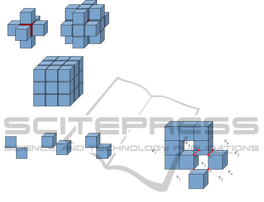
(a) 6-adjacency (b) 18-adjacency
(c) 26-adjacency
Figure 1: Kinds of adjacency of a voxel with its local neigh-
borhood.
Figure 2: Non-manifold 2D (left) and 3D (middle and right)
configurations.
χ = n
0
− n
1
+ n
2
− n
3
(1)
where n
0
, n
1
, n
2
and n
3
are, respectively, the num-
ber of vertices (points), edges (linear elements), faces
(surfels) and voxels of the voxel model. This expres-
sion can be applied to several adjacency pairs (Tori-
waki and Yonekura, 2002). In the solid modeling
field, χ can also be computed from a polyhedronusing
the following expression (Mantyla, 1988):
χ = V − E + F − R (2)
where V, E, F and R are, respectively, the number of
vertices, edges, faces and internal rings of faces. This
expression can also be applied to triangular surfaces,
F being the number of triangles and R = 0. From
the theory of homology, the Euler-Poincar´e formula
relates χ with the Betti numbers h
i
(Massey, 1991):
χ = h
0
− h
1
+ h
2
(3)
where h
0
, h
1
and h
2
are, respectively, the number of
connected components, the connectivity and the num-
ber of isolated cavities. h
0
and h
2
are usually com-
puted using CCL-based methods over voxels, poly-
hedron faces or triangles, depending on the model
used. Then, the connectivity h
1
which is related to
the genus, can be computed from χ, h
0
and h
2
using
Expression 3.
Although binary volumes with adjacency pairs (6,
26) or (26, 6) are non-manifold, χ and the genus can
be computed unambiguously for them. When com-
puting n
0
and n
1
in Expression 1 the adjacency pair
is taken into consideration in such a way that non-
manifold edges and vertices are counted once for 26-
adjacency and twice for 6-adjacency. For example, in
the case of the object depicted in Figure 3, consid-
ering the adjacency pair (26, 6), the number of con-
nected components (h
0
) is 1 and vertices v
1
to v
6
and
edges e
1
, e
2
are counted just once because they belong
to two connected voxels, so, the genus (h
1
), which can
be seen as the number of handles, is 2. But consider-
ing the adjacency pair (6, 26), h
0
= 3 and in this case
the vertices v
1
to v
6
and edges e
1
, e
2
must be counting
twice because they belong to separating two voxels,
giving a genus=0.
Figure 3: Illustrative figure consisting of 9 voxels for calcu-
lating the genus depending on the selected adjacency pair.
A binary volume dataset can be represented in a
compact way by an OP (Khachan et al., 2000). Based
on this fact, a previous approach (Ayala et al., 2012)
computes χ and the genus of a binary volume dataset
using expression 2. In this method, the binary vol-
ume dataset is represented with a model suitable for
OP and when the object presents non-manifold con-
figurations, it needs to be converted into an homo-
topic manifold analog. This approach has proved to
be more efficient than methods based on voxel mod-
els and triangle meshes.
Expression 2 and 3 are used to compute the con-
nectivity of a triangular mesh representing some ade-
nine properties in the biochemistry field (Konkle
et al., 2003). In isosurface extraction, the topology-
preservation is sometimes a desirable property that
can be evaluated by computing χ (Schaefer et al.,
2007). In the Bio-CAD field, the connectivity is re-
lated to biomechanical properties and is used to mea-
sure the strength of bone or other materials. The
method based on Expressions 1 and 3 is used to eval-
uate the osteoporosis degree of mice femur (Mart´ın-
Badosa et al., 2003) or human vertebrae (Odgaard and
Gundersen, 1993) or to evaluate hydraulic properties
AnEfficientAlternativetoComputetheGenusofBinaryVolumeModels
19

of sintered glass (Vogel et al., 2005).
Binary volume models are mostly represented
with the classical voxel model. However, for specific
purposes, several alternative models have been de-
vised. Hierarchical decomposition models as octrees
and kd-trees have been used for Boolean operations
(Samet, 1990), CCL (Dillencourt et al., 1992) and
isosurface extraction (And´ujar et al., 2002; Vander-
hyde and Szymczak, 2008). Other models store only
surface voxels to improve spatial or querying perfor-
mance, such as the semi-boundary (Grevera et al.,
2000) and the slice-based binary shell representation
(Kim et al., 2001).
In this work we represent a binary volume with a
decomposition model, the Compact Union of Disjoint
Boxes (CUDB). This model is suitable for binary vol-
umes as well as for OP and is introduced in the next
section. Section 4 presents our approach to compute
χ and the genus of a binary volume. The first con-
tribution is a method to compute χ, that applies Ex-
pression 1 to each box of the CUDB, taking into ac-
count the overlapping regions among boxes. The sec-
ond contribution is a CCL-based method that obtains
the connected components and cavities of the object
in order to compute the connectivity from Expression
3. Section 5 presents the results obtained with sev-
eral phantom and real datasets, besides, we also com-
pare the performance of our method with the methods
based respectively on the voxel model (Toriwaki and
Yonekura, 2002) and on OP (Ayala et al., 2012). Fi-
nally, Section 6 concludes this paper.
3 THE CUDB MODEL
To introduce the Compact Union of Disjoint Boxes
(CUDB) model, we will consider the pseudo-
manifold orthogonal polyhedron (OP) that constitutes
the continuous analog of the binary voxel model.
Let P be an OP and Π
c
a plane whose normal
is parallel, without loss of generality, to the X axis,
intersecting it at x = c, where c ranges from −∞
to +∞. Then, this plane sweeps the whole space
as c varies within its range, intersecting P at cer-
tain intervals. Let us assume that this intersection
changes at c = C
1
,...,C
n
. More formally, P∩Π
C
i
−δ
6=
P∩Π
C
i
+δ
,∀i = 1,..., n, where δ is an arbitrarily small
quantity. Then, C
i
(P) = P∩ Π
c
i
is called a cut of P
and S
i
(P) = P ∩ Π
C
s
, for any C
s
such that C
i
< C
s
<
C
i+1
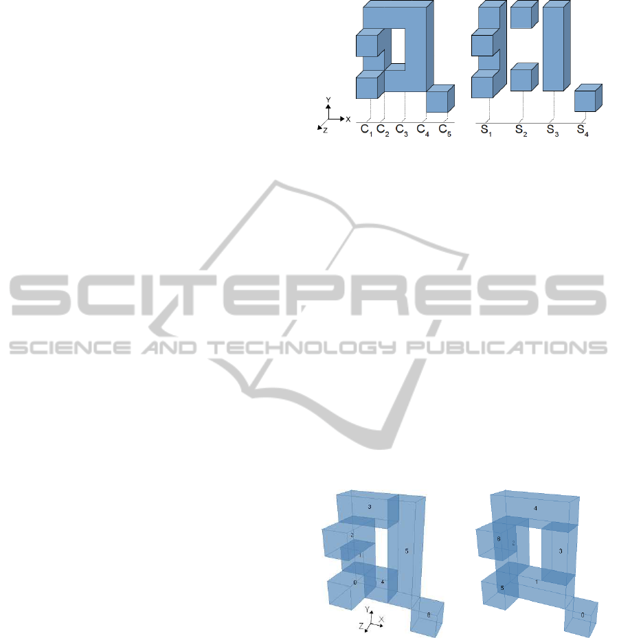
, is called a section of P. Figure 4 shows an OP
with its cuts and sections perpendicular to the X axis.
Since we work with bounded regions, S
0
(P) =
/
0 and
S
n
(P) =
/
0, where n is the total number of cuts along a
given coordinate axis.
Figure 4: Left: an orthogonal polyhedron with 5 cuts.
Right: its sequence of 4 prisms with the representative sec-
tions (X direction).
An OP can be represented with a sequence of or-
thogonal prisms represented by their section. More-
over, if we apply the same reasoning to the represen-
tative section of each prism, an OP can be represented
as a sequence of boxes. CUDB represents an OP with
such an ordered sequence of boxes in a compact way,
as many boxes generated by the aforementioned split
process are merged into one in several parts of the
model. CUDB is axis-aligned like octrees and bin-
trees, but the partition is done along the object geom-
etry as in binary space partitioning (BSP). Depend-
ing on the order of the axes along which we choose
to split the data, an object can be decomposed into
six different sets of boxes: XYZ, XZY, YXZ, YZX,
ZXY, ZYX, and the set will be ordered according to
the chosen configuration. Figure 5 illustrates two pos-
sible decompositions of the model in Figure 4 (left).
Figure 5: XYZ-CUDB (left) and ZYX-CUDB (right) rep-
resentation for the model in Figure 4, both with 7 boxes.
In the CUDB model, the adjacency information
(either 6 or 26-adjacency) of the boxes is stored. Each
box has neighboring boxes in only two orthogonal di-
rections, i.e., for a given ABC-ordering, a box can
have neighbors only in A and B direction, and each
direction goes in two opposite ways. Thus, there
are 4 arrays (2 for each direction) of pointers to the
neighboring boxes. For more details of this model see
(Cruz-Mat´ıas and Ayala, 2011) and (Rodr´ıguez et al.,
2011).
GRAPP2013-InternationalConferenceonComputerGraphicsTheoryandApplications
20

4 CONNECTIVITY
COMPUTATION
The approach followed in this paper to compute the
Euler characteristic and the genus is based on Expres-
sion 1, and considers a box as a rectangular prism en-
closing a finite number of voxels. In the voxel model,
a simple way to compute the number of faces, edges
and vertices reported for each voxel when Expression
1 is used, is by checking the lower 13 neighbors (N
−
)
of the voxelfor a backward scan, where the 6 faces, 12
edges and 8 vertices of each visited voxel are added
and the possible shared elements (3 faces, 9 edges and
7 vertices) are subtracted. An analogy to this reason-
ing is used in our approach.
Let β be a box in the CUDB model, β is repre-
sented by two diagonally opposed vertices~v
0
and~v
1
,
the ones with lesser and greater coordinate values re-
spectively, where
~
d =~v
1
−~v
0
= (d
x
,d
y
,d
z
) represents
the main diagonal vector of β and d
x
, d
y
and d
z
its di-
mensions. Then, for any box β in the CUDB model,
the number of enclosed voxels (γ
β
), faces (f
β
), edges
(e
β
) and vertices (v
β
) are computed as:
γ
β
= d
x
· d
y
· d
z
(4)
f
β
= [d
x
· d
y
· (d
z
+ 1)] + [d
x
· (d
y
+ 1) · d
z
]
+[(d
x
+ 1) · d
y
· d
z
] (5)
e
β
= [d
x
· (d
y
+ 1) · (d
z
+ 1)]
+[(d
x
+ 1) · d
y
· (d
z
+ 1)] + [(d
x
+ 1) · (d
y
+ 1) · d
z
] (6)
v
β
= (d
x
+ 1) · (d
y
+ 1) · (d
z
+ 1) (7)
After computing the enclosed unitary elements of
β, we have to analyze its backward neighbors (BN),
in order to subtract the elements reported by the over-
lapping regions. For simplicity we consider the XYZ-
ordering, therefore, as we said in Section 3, a box can
have neighbors only in X and Y direction, so, just the
BN in this directions need to be checked.
At this point it is important to say that, indepen-
dently of the used adjacency pair, (26, 6) or (6, 26),
in the binary volume model, our method requires the
CUDB with the neighboring boxes information ac-
cording to 26-adjacency. This is because if we con-
sider a CUDB with 6-adjacency, the connected com-
ponents still have boxes with overlapping regions that
are 26-adjacent, which must be considered in the ele-
ments subtraction (e.g. see the boxes 1 and 4 in Fig-
ure 5 (left)). Therefore, in order to compute χ and
genus for a (6, 26) binary volume model, we simply
obtain the connected components of the foreground
according to 6-adjacency and then, each of them is
separately analyzed with 26-adjacency to count the
enclosed elements. For now on we suppose the case
of the (26, 6) adjacency pair.
In CUDB when considering26-adjacency, it is im-
portant to notice that two edge-adjacent boxes β
i
and
β
k
are neighbors only in one direction, i.e. if the over-
lapping region between β
i
and β
k
is a segment (part
of an edge), when it is Y or Z-aligned, β
i
and β
k
are
neighbors in X-direction, and when the segment is X-
aligned, β
i
and β
k
are neighbors in Y-direction. If the
overlapping region between β
i
and β
k
is a vertex, then
they are neighbors just in X-direction. For example,
in the configurations depicted in Figure 2 (middle and
right), the boxes are neighbors in X-direction in both
cases.
The method performs a traversal of CUDB and for
each box B, computes its unitary elements (γ
β
, f
β
, e
β
,
v
β
) according to Expressions 4 to 7. However, there
are overlapping regions among boxes and the method
must deal correctly with them.
4.1 Shared Elements Computation
Overlapping regions can be rectangles (2D), line seg-
ments (1D) (segments from now on) or points (0D).
They have to be detected and their contribution com-
puted and added or subtracted to the global value.
A box β
i
shares a rectangle R with any backward
neighbor in X (X-BN) and in Y-direction (Y-BN) (see
Figure 6(a) and (b) in red). The basic unitary ele-
ments enclosed by this rectangle are computed twice
and therefore we have to subtract them once. Let r
x
and r
y
be the dimensions of R, the faces (f
R
), edges
(e
R
) and vertices (v
R
) can be be computed in a way
similar to that of Expressions 5 to 7:
f
R
= r
x
· r
y
(8)
e
R
= r
x
· (r
y
+ 1) + (r
x
+ 1) · r
y
(9)
v
R
= (r
x
+ 1) · (r
y
+ 1) (10)
However, more than one BN can share a segment
with β
i
. We have performed an exhaustive case study
of the overlapping regions by analyzing the possi-
ble neighborings among boxes in the CUDB model.
There can be 1, 2 or 3 backward neighboring boxes
that share a segment with β
i
.
In the first case only the shared rectangle must be
computed and subtracted as discussed above. Note
that in some cases a degenerated rectangle is obtained
(see boxes β
i
and β
x
in Figure 6(d)).
In the case of two BN of β
i
sharing a segment
S, it has been subtracted twice and therefore it must
be added again. For example, in Figure 6(c) the red
regions computed when analyzing the pairs of boxes
(β
i
,β
x
) and (β
i
,β
t
) have been subtracted and there-
fore the yellow region has been subtracted twice and
has to be added again. There are 4 possible configu-
rations for two BN of β
i
sharing a segment.
AnEfficientAlternativetoComputetheGenusofBinaryVolumeModels
21

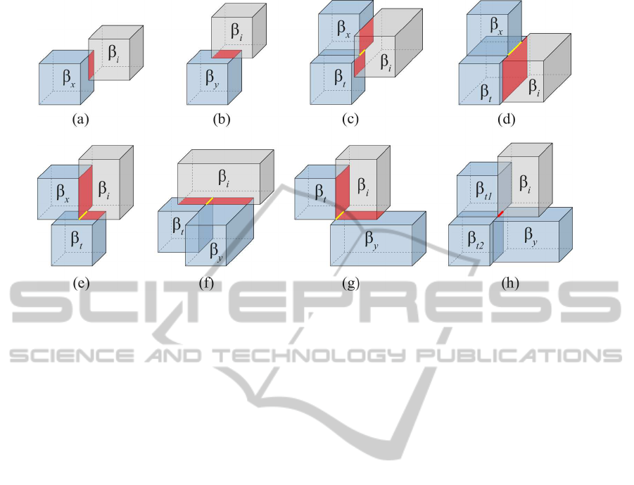
Figure 6: Backward neighbors(BN) configurations of a box β
i
. (a) A X-BN sharing a rectangle. (b) A Y-BN sharing a
rectangle. (c) Two X-BN sharing a segment. (d) degenerated case of (c). (e) A X and a Y-BN sharing a segment. (f) Two
Y-BN sharing a segment. (g) A Y and a X-BN sharing a segment. (h) A Y and two X-BN sharing a segment.
C1. Two X-BN (β
x
and β
t
), where β
t
is Y-BN of β
x
.
See Figure 6(c and d).
C2. One X-BN (β
x
) and one Y-BN (β
t
), where β
t
is
Y-BN of β
x
. See Figures 6(e).
C3. Two Y-BN (β
y
and β
t
), where β
t
is X-BN of β
y
.
See Figure 6(f).
C4. One Y-BN (β
y
) and one X-BN (β
t
), where β
t
is
X-BN of β
y
. See Figure 6(g).
Then, if s is the length of S, the enclosed unitary edges
(e
S
) and vertices (v
S
) of S are computed as:
e
S
= s, v
S
= s+ 1 (11)
In the case of three BN of β
i
sharing a segment S,
there is only one possible configuration:
C5. One Y-BN (β
y
) and two X-BN (β
t1
and β
t2
),
where both β
t1
and β
t2
are X-BN of β
y
and Y-
neighbors between them. See Figure 6(h).
Note that configuration C5 is equivalent to two
occurrences of C1 ((β
y
,β
t1
,β
t2
) and (β
i
,β
t1
,β
t2
)) and
two occurrences of C4 ((β
i
,β
y
,β
t1
) and (β
i
,β
y
,β
t2
)).
However, both configurations C4 occur when β
i
is
being analyzed and, therefore, some shared elements
with β
t1
in one occurrence and with β
t2
in the other,
are added twice, so, the shared segment S by β
i
, β
t1
and β
t2
(highlighted in red in Figure 6(h)), represents
the region that must be re-subtracted. The enclosed
unitary edges (e
S
) and vertices (v
S
) are computed as
in Expression 11. This case is solved by inserting all
the β
t
of configurations C4 into a list and then the list
is analyzed in order to check for boxes that are Y-BN.
4.2 Connected Component Labeling
For the CCL process, we have followed the classi-
cal two-pass strategy of first labeling and then renum-
bering a set of equivalences (Wu et al., 2009). As
we have the neighbors of each box, we avoid the
neighborhood test. In our labeling process the CUDB
model is traversed and, on the fly, each box β
i
is la-
beled with the minimum value of its already labeled
BN, or with a new label if it doesn’t have labeled
BN. When β
i
has two or more labeled BN with dif-
ferent values, a label equivalence is recorded into a
map, where the key value corresponds to the region
number and the mapped value to its label. All the
equivalences are solved in the renumbering pass that
first sorts out all the equivalences and then propagates
them correctly. As a result, we get the number of con-
nected components.
As both the connectivity computation and the
CCL processes require a traversal of the boxes and
its BN, we have merged both algorithms into one.
The proposed method uses the CUDB representation
(CUDB-Rep) of an OP that has already been com-
puted. The next pseudo-code represents the whole
process.
Input: CUDB-Rep of the OP.
Output: Euler characteristic (χ) and genus.
1. currentLabel = n
0
= n
1
= n
2
= n
3
= 0.
2. For each box, β
i
,i = 1..n, in the CUDB-Rep do:
A. Compute γ
i
, f
i
, e
i
, v
i
.
GRAPP2013-InternationalConferenceonComputerGraphicsTheoryandApplications
22

B. Do mlabel = ∞.
C. for each X-BN β
x
do:
i. if β
x
.label < mlabel then, mlabel = β
x
.label
ii. Compute f
R
, e
R
and v
R
.
iii. Do f
i
–=f
R
, e
i
–=e
R
and v
i
–=v
R
s.
iv. for each X-BN, β
t
do: //Configurations C1
(a) if β
t
is Y-BN of β
x
, then, compute e
S
and
v
S
, and do e
i
+=e
S
and v
i
+=v
S
.
v. for each Y-BN, β
t
do: //Configurations C2
(a) if β
t
is Y-BN of β
x
, then, compute e
S
and
v
S
, and do e
i
+=e
S
and v
i
+=v
S
.
D. for each Y-BN, β
y
do:
i. if β
y
.label < mlabel then, mlabel = β
y
.label
ii. Compute f
R
, e
R
and v
R
.
iii. Do f
i
–=f
R
, e
i
–=e
R
and v
i
–=v
R
.
iv. for each Y-BN, β
t
do: //Configurations C3
(a) if β
t
is X-BN of β
y
, then, compute e
S
and v
S
, and do e
i
+=e
S
and v
i
+=v
S
.
v. Create a list of boxes L.
vi. for each X-BN, β
t
do: //Configurations C4
(a) if β
t
is X-BN of β
y
, then, compute e
S
and v
S
, do e
i
+=e
S
and v
i
+=v
S
and insert
β
t
to L.
vii. for each pair (β
t1
, β
t2
) in L which are Y-
neighbors do: //Configurations C5
(a) Compute e
S
and v
S
.
(b) Do e
i
–=e
S
and v
i
–=v
S
.
E. Do n
0
+=v
i
, n
1
+=e
i
, n
2
+=f
i
, and n
3
+=γ
i
.
F. if mlabel = ∞ then
i. Do mlabel = currentLabel.
ii. Do currentLabel++.
G. for each X-BN and Y-BN, β
t
do:
i. if β
t
is labeled, then, add equivalence
β
t
.label = mlabel into the map equivalences.
ii. else do β
t
.label= mlabel.
3. Do χ = n
0
− n
1
+ n
2
− n
3
.
4. Number of cc (h
0
) = renumbering(equivalences).
5. Compute the complement of CUDB-Rep.
6. Number of cavities (h
2
) = CCL(complement)-1.
7. Do genus(h
1
) = h
0
+ h
2
− χ.
Step 2 computes the same number of voxels,
faces, edges and vertices that the voxel-based method
and simultaneously performs the first step of the CCL
process. Step 3 computes χ using Expression 1. Step
4 performs the CCL relabeling process, which returns
the number of connected components. Step 6 applies
our standard version of CUDB-based CCL to com-
pute the number of internal cavities (the connected
components of the object complement). Finally, step
7 computes the genus using Expression 3.
5 RESULTS
We have measured χ and the genus for a selection of
datasets with different shape features and size. They
present non-manifold configurations and may contain
isolated cavities and disconnected components. Fig-
ure 7 shows rendered views of the test datasets and its
size in the voxel model, where from (j) to (r) are real
volume data coming from CT or MRI scanners. These
datasets come from public volume repositories. Three
methods have been compared: voxel-based, OP-based
(see Section 2) and CUDB-based, presented in this
paper. These methods produce exactly the same re-
sults. The algorithms has been written in C++ and
tested on a PC Intel
R
Core 2 E6600 at 2.4 GHz with
3.2 Gb RAM under Linux.
We work on a platform where the main represen-
tation models are CUDB and the Extreme Vertices
Model (EVM), which is a very concise B-Rep model
for OP with very fast Boolean operations. EVM can
be obtained from the voxel model, in turn, CUDB
is obtained from EVM. The conversions algorithms
have been published (Aguilera, 1998; Cruz-Mat´ıas
and Ayala, 2011). These models are used in other
processes in diverse research topics, so, we consider
that they are available and ignore the cost of conver-
sion from the voxel model, similar to the OP-based
method. Thus, to compute the complement of the in-
put model, we use the EVM representation, whose
runtime is negligible. However, the conversion time
of the complement to CUDB is considered in our
computation times (step 5 of the algorithm).
Table 1 shows the attributes of the tested datasets:
number of foreground voxels, number of boxes in
their CUDB-Rep, number of connected components
(C
+
), number of isolated cavities (C
−
), χ and genus
using the adjacency pair (26, 6).
Table 2 shows the required time in seconds to
compute χ and the genus for each referenced method.
To compute the genus, the three methods need to com-
pute the complement of the model, and besides, the
OP-based method needs to convert the OP to a homo-
topic manifold analog. Note that our proposal is very
fast to compute χ, and regarding the genus computa-
tion, it is by far, faster than the voxel-based method, in
some datasets up to two orders of magnitude (pelvis,
golfBall, pegasus, aneurysm and beetle). Compared
to the previous OP-based our method is also faster in
all the tested datasets, in some of them up to an order
of magnitude (pegasus, teddy and femur). Moreover,
we report the conversion times: voxel to EVM (tc
1
)
and EVM to CUDB (tc
2
) in order to show that, even
considering these costs, the overall time (t
o
) of our
method is better than the voxel-based method.
AnEfficientAlternativetoComputetheGenusofBinaryVolumeModels
23

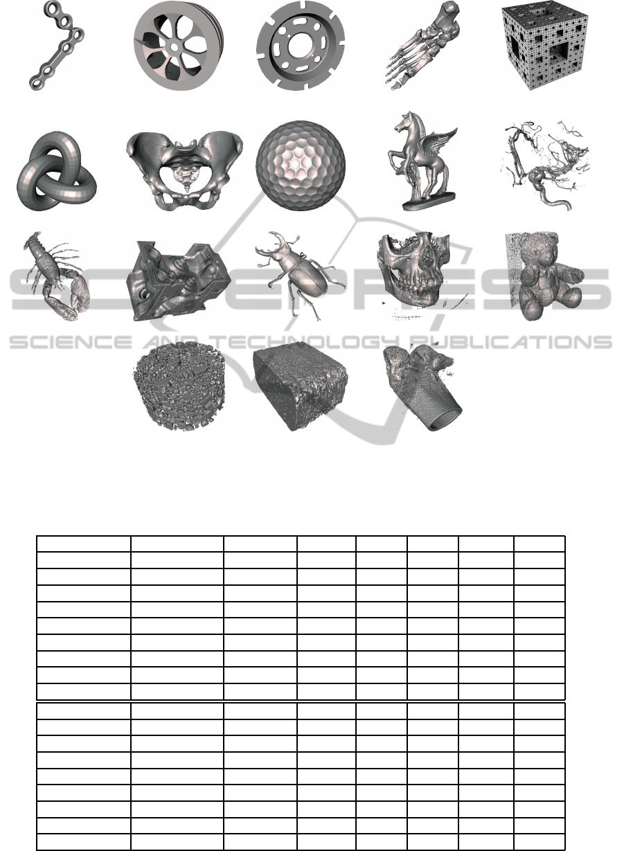
(a) Tool (b) Wheel (c) DiskBrake (d) Foot (e) Menger- 4
(f) Knot (g) Pelvis (h) GolfBall (i) Pegasus (j) Aneurysm
(k) Lobster (l) Engine (m) Beetle (n) Skull (o) Teddy
(p) Mineral (q) Rock (r) Femur
Figure 7: Rendered images of the test datasets.
Table 1: Attributes of the test datasets. For each dataset, the size of the voxel model, number of foreground voxels, number
of boxes in its CUDB-Rep. Next, with an adjacency pair (26,6): the number of connected components, number of isolated
cavities, the Euler characteristic χ and genus.
Dataset size # for. vox. # boxes C
+
C
−
χ genus
(a) Tool 511x339x48 1778611 11000 1 0 -10 6
(b) Wheel 120x300x300 3809958 13207 1 0 -14 8
(c) DiskBrake 511x512x73 2584762 29516 1 0 -20 11
(d) Foot 183x512x185 1818019 35498 6 24 -86 73
(e) Menger-4 162x162x162 1280000 46704 1 0 -52864 26433
(f) Knot 329x350x257 7509337 76831 1 0 0 1
(g) Pelvis 368x512x450 5920950 85923 1 8 -10 14
(h) GolfBall 510x509x511 13645424 129493 1 0 2 0
(i) Pegasus 598x800x574 24683709 191747 1 8 2 8
(j) Aneurysm 213x215x240 69743 10705 406 12 544 146
(k) Lobster 244x239x49 233509 19322 53 180 -638 552
(l) Engine 139x197x108 901818 25524 9 194 146 130
(m) Beetle 411x371x247 1737343 36052 17 114 -190 226
(n) Skull 256x256x256 1112906 114563 1624 337 -1020 2471
(o) Teddy 424x321x493 24758866 124063 59 212 -2580 1561
(p) Mineral 376x375x206 7363953 232008 724 5 -2792 2125
(q) Rock 240x406x267 19348939 331491 1336 17263 25828 5685
(r) Femur 463x494x628 4014089 838585 22714 7909 -25144 43195
GRAPP2013-InternationalConferenceonComputerGraphicsTheoryandApplications
24

Table 2: Statistics of the test dataset. For each dataset the computation time in seconds for the voxel-based (mvx), OP-based
and the CUDB-based methods. The last columns represent the conversion times: voxel to EVM (tc
1
) and EVM to CUDB
(tc
2
) of the original model, t
o
= tc
1
+tc
2
+CUDB
∗
.
Dataset
Time χ Total time (genus)
tc
1
tc
2
t
o
mvx OP CUDB mvx OP CUDB
∗
(a) Tool 1.77 0.26 0.01 6.22 0.84 0.11 1.47 0.13 1.71
(b) Wheel 3.84 0.24 0.01 10.84 1.47 0.20 2.60 0.20 3.00
(c) DiskBrake 4.94 0.81 0.01 17.09 2.42 0.28 5.24 0.22 5.73
(d) Foot 7.72 0.79 0.02 22.22 2.45 0.29 4.58 0.25 5.13
(e) Menger-4 1.30 0.70 0.02 3.85 1.52 0.27 1.05 0.21 1.53
(f) Knot 9.19 1.94 0.05 29.07 5.83 0.64 1.94 0.49 3.06
(g) Pelvis 26.81 2.16 0.06 101.21 6.93 0.71 23.33 0.55 24.59
(h) GolfBall 41.53 2.90 0.07 150.37 9.49 1.20 34.72 0.89 36.81
(i) Pegasus 71.54 6.15 0.13 274.83 20.81 1.88 72.82 1.46 76.16
(j) Aneurysm 2.99 0.37 0.01 10.26 0.92 0.10 2.57 0.08 2.75
(k) Lobster 0.61 0.49 0.02 2.14 1.31 0.16 0.63 0.13 0.92
(l) Engine 0.77 0.62 0.02 2.43 1.77 0.21 0.71 0.16 1.07
(m) Beetle 11.08 2.01 0.02 39.39 2.34 0.29 9.49 0.25 10.03
(n) Skull 5.74 3.51 0.06 19.40 9.16 0.94 5.10 0.68 6.71
(o) Teddy 20.97 3.49 0.09 74.07 10.39 1.02 18.23 0.77 20.01
(p) Mineral 9.35 5.92 0.16 31.04 19.25 1.97 8.76 1.48 12.22
(q) Rock 12.48 9.47 0.39 33.89 24.43 3.44 8.65 1.93 14.01
(r) Femur 45.94 31.16 0.80 170.64 80.66 8.06 41.90 5.69 55.65
6 CONCLUSIONS AND FUTURE
WORK
We have presented a method to compute the Euler
characteristic and the genus of binary volume datasets
using the CUDB model, and we have evaluated its
performance compared to existing methods applied to
voxel models and OP. We have tested several public
volume datasets, both phantom and real. We conclude
that computing the connectivity is notably faster in
our approach. The performance variability is caused
by the dataset size but above all to their surface in-
tricacy: the voxel-based method performance is func-
tion of the number of voxels, but our method depends
on the number of boxes, tightly related to the model’s
tortuosity (a property that represents the twist of a
curve, i.e. the degree of turns or detours a model
has (Grisan et al., 2003)), like the previous developed
methods based on OP.
As future work, we plan to study a method to
compute the complement of a model directly from its
CUDB-Rep, in order to leave aside the EVM repre-
sentation, since, as can be seen in Table 2, the differ-
ence in time to compute χ and genus is mainly due
to the conversion of the complement from EVM to
CUDB. Furthermore, in the biomedical field, there
are other structural parameters that can be studied to
describe properties of a biomaterial, in this field we
have used the CUDB model in a method to simulate
the mercury intrusion in a porous medium (Rodr´ıguez
et al., 2011). At present, we are beginning to study
simplification (Cruz-Mat´ıas and Ayala, 2012) and
time-varying techniques based on EVM and CUDB
models.
ACKNOWLEDGEMENTS
This work was partially supported by the national
projects TIN2008-02903 and TIN2011-24220 and a
MAEC-AECID grant for I. Cruz-Mat´ıas, all of the
Spanish government. The authors thank the anony-
mous reviewers whose remarks and suggestions have
allowed to greatly improve the paper.
REFERENCES
Aguilera, A. (1998). Orthogonal Polyhedra: Study and Ap-
plication. PhD thesis, LSI-UPC.
And´ujar, C., Brunet, P., and Ayala, D. (2002). Topology-
reducing surface simplification using a discrete solid
rep. ACM Trans. on Graphics, 21(2):88 – 105.
Ayala, D., Verg´es, E., and Cruz, I. (2012). A polyhedral
approach to compute the genus of a volume dataset. In
Proceedings of the GRAPP 2012, pages 38–47, Rome,
Italy. INSTICC Press.
AnEfficientAlternativetoComputetheGenusofBinaryVolumeModels
25

Cruz-Mat´ıas, I. and Ayala, D. (2011). CUDB: An im-
proved decomposition model for orthogonal pseudo-
polyhedra. Technical Report LSI-11-2-T, UPC.
Cruz-Mat´ıas, I. and Ayala, D. (2012). Orthogonal simplifi-
cation of objects represented by the extreme vertices
model. In Proceedings of the GRAPP 2012, pages
193–196, Rome, Italy. INSTICC Press.
Dillencourt, M., Samet, H., and Tamminen, M. (1992).
A general approach to connected-component labeling
for arbitrary image representations. Journal of the
ACM, 39(2):253 – 280.
Grevera, G. J., Udupa, J. K., and Odhner, D. (2000). An
order of magnitude faster isosurface rendering in soft-
ware on a PC than using dedicated, GP rendering
hardware. IEEE Trans. Vis. and CG., 6(4):335–345.
Grisan, E., Foracchia, M., and Ruggeri, A. (2003). A novel
method for the automatic evaluation of retinal vessel
tortuosity. In Proc. of the 25th Annual Int. Conf. of the
IEEE EMBS, 2003., volume 1, pages 866 – 869 Vol.1.
Khachan, M., Chenin, P., and Deddi, H. (2000). Polyhedral
representation and adjacency graph in n-dimensional
digital images. Computer Vision and Image under-
standing, 79:428 – 441.
Kim, B., Seo, J., and Shin, Y. (2001). Binary volume render-
ing using Slice-based Binary Shell. The Visual Com-
puter, 17:243 – 257.
Kong, T. and Rosenfeld, A. (1989). Digital topology: Intro-
duction and survey. Computer Vision, Graphics and
Image Processing, 48:357–393.
Konkle, S., Moran, P., Hamann, B., and Joy, K. (2003). Fast
methods for computing isosurface topology with Betti
numbers. In Data Visualization, pages 363 – 376.
Lachaud, J. and Montanvert, A. (2000). Continuous analogs
of digital boundaries: A topological approach to iso-
surfaces. Graphical Models, 62:129 – 164.
Latecki, L. (1997). 3D Well-Composed Pictures. Graphical
Models and Image Processing, 59(3):164–172.
Latecki, L., Eckhardt, U., and Rosenfeld, A. (1995). Well-
composed sets. Computer Vision and Image Under-
standing, 61(1):70–83.
Mantyla, M. (1988). An Introduction to Solid Modeling.
Computer Science Press.
Mart´ın-Badosa, E., Elmoutaouakkil, A., Nuzzo, S., Am-
blard, D., Vico, L., and Peyrin, F. (2003). A method
for the automatic characterization of bone architecture
in 3D mice microtomographic images. Computerized
Medical Imaging and Graphics, 27:447–458.
Massey, W. S. (1991). A Basic Course in Algebraic Topol-
ogy. Springer-Verlag.
Odgaard, A. and Gundersen, H. J. (1993). Quantification of
Connectivity in Cancellous Bone, with Special Em-
phasis on 3-D Reconstructions. Bone, 14:173 – 182.
Rodr´ıguez, J., Cruz, I., Verg´es, E., and Ayala, D. (2011). A
connected-component-labeling-based approach to vir-
tual porosimetry. Graphical Models, 73:296–310.
Samet, H. (1990). Applications of spatial data struc-
tures: Computer graphics, image processing, and
GIS. Addison-Wesley Longman Publishing Co., Inc.
Schaefer, S., Ju, T., and Warren, J. (2007). Manifold dual
contouring. IEEE Transactions on Visualization and
Computer Graphics, 13(3):610 – 619.
Toriwaki, J. and Yonekura, T. (2002). Euler number and
connectivity indexes of a three dimensional digital
picture. Forma, 17:183–209.
Vanderhyde, J. and Szymczak, A. (2008). Topological sim-
plification of isosurfaces in volume data using octrees.
Graphical Models, 70:16 – 31.
Vogel, H. J., T¨olke, J., Schulz, V., Krafczyk, M., and Roth,
K. (2005). Comparison of a lattice-boltzmann model,
a full-morphology model, and a pore network model
for determining capillary pressure-saturation relation-
ships. Vadose Zone Journal, 4:380 –388.
Wu, K., Otoo, E., and Suzuki, K. (2009). Optimizing two-
pass connected-component labeling algorithms. Pat-
tern Anal. Appl., 12(2):117–135.
GRAPP2013-InternationalConferenceonComputerGraphicsTheoryandApplications
26