
Real-time Multiple Abnormality Detection in Video Data
Simon Hartmann Have, Huamin Ren and Thomas B. Moeslund
Visual Analysis of People Lab, Aalborg University, Aalborg, Denmark
Keywords:
Abnormality Detection, Cascade Classifier, Video Surveillance, Optical Flow.
Abstract:
Automatic abnormality detection in video sequences has recently gained an increasing attention within the
research community. Although progress has been seen, there are still some limitations in current research.
While most systems are designed at detecting specific abnormality, others which are capable of detecting
more than two types of abnormalities rely on heavy computation. Therefore, we provide a framework for
detecting abnormalities in video surveillance by using multiple features and cascade classifiers, yet achieve
above real-time processing speed. Experimental results on two datasets show that the proposed framework
can reliably detect abnormalities in the video sequence, outperforming the current state-of-the-art methods.
1 INTRODUCTION
Abnormality detection is an important problem that
has been researched within diverse research areas and
application domains. Many abnormality detection
techniques have been specially developed for certain
application domains, e.g. car counting (Stauffer and
Grimson, 2000), group activity detection (Cui et al.,
2011), monitoring vehicles (Yu and Medioni, 2009)
etc. A key issue when designing an abnormality de-
tector is how to represent the data in which anoma-
lies are to be found. Considering approaches in the
context of video surveillance, existing methods in the
literature can be classified into two categories:
1) Data analysis by tracking, in which objects are
represented by trajectories. A commonly used ap-
proach is based on obtained clusters of the trajectories
for moving objects, which are later used as an abnor-
mality model. Johnson et al. (Johnson and Hogg,
1995) were probably among the first researches in
this direction, they used vector quantization to ob-
tain a compact representation of trajectories and uti-
lized multilayer neural networks for the identification
of common patterns. Piciarelli et al. (Piciarelli and
Foresti, 2006) proposed a trajectory clustering algo-
rithm especially suited for online abnormality detec-
tion. Hu et al. (Hu et al., 2006) hierarchically clus-
tered trajectories depending on spatial and temporal
information. While trajectory based approaches are
suitable in scenes with few objects, they cannot main-
tain reliable tracks in crowded environments due to
occlusion and overlap of objects (Mahadevan et al.,
2010).
2) Data analysis without tracking, in which fea-
tures such as motion or texture are extracted to model
activity patterns of a given scene. Different features
have been attempted. For example, Mehran et al.
(Mehran et al., 2009) modeled crowd behavior using
a ”social force” model, where the interaction forces
were computed using optical flow. (Mahadevan et al.,
2010) recently proposed mixtures of dynamic tex-
tures to jointly model the appearance and dynamics
of crowded scenes, to address the problem of abnor-
mality detection with size or appearance variation in
objects. (Zhao et al., 2011) provided a framework of
using sparse coding and online re-constructibility to
detect unusual events in videos.
Although progress has been made, there are still
some limitations in current research: while most sys-
tems are designed at detecting specific abnormality,
others which are capable of detecting more than two
types of abnormalities rely on heavy computation. In
this work, we provide a framework of using multiple
features and cascade classifiers to detect several ab-
normal activities in videos yet achieve real-time pro-
cessing speed.
2 PROPOSED METHOD
Two important criteria to evaluate abnormality detec-
tion systems are time response and types of abnor-
malities that can be detected. To meet the require-
ments of a practical abnormality detection system, our
390
Have S., Ren H. and Moeslund T..
Real-time Multiple Abnormality Detection in Video Data.
DOI: 10.5220/0004280703900395
In Proceedings of the International Conference on Computer Vision Theory and Applications (VISAPP-2013), pages 390-395
ISBN: 978-989-8565-48-8
Copyright
c
2013 SCITEPRESS (Science and Technology Publications, Lda.)
system is designed to detect multiple unusual events.
To attain this goal, we adopt four types of features,
train their corresponding classifiers, and cascade these
classifiers to determine if the query video contains ab-
normality or not.
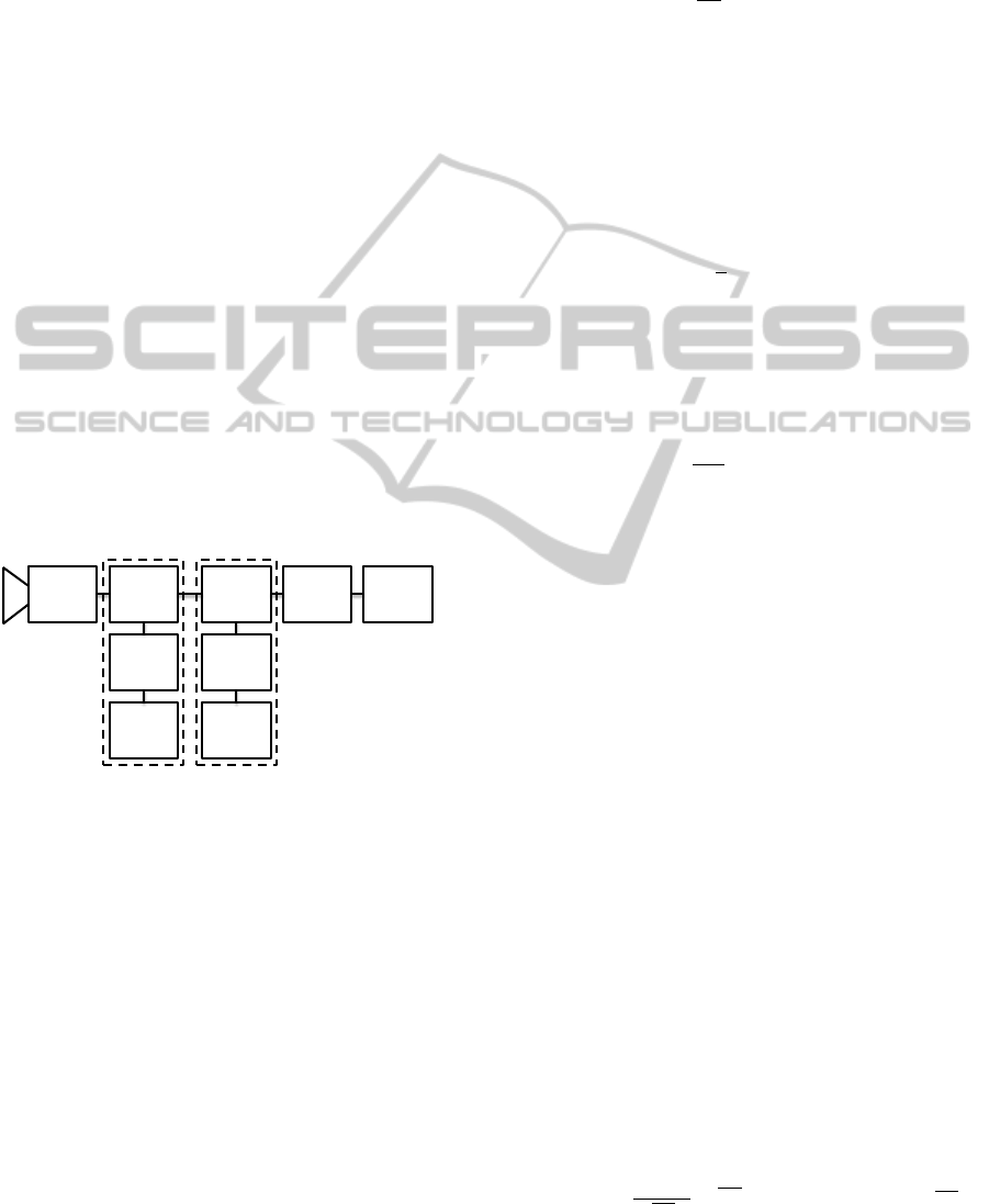
2.1 System Overview
An overview of our system is illustrated in Figure 1.
A figure-ground segmentation is carried out to extract
foreground pixels. This not only allows for using ob-
ject size as a feature, but also reduces the aperture
problem related to image motion detection via opti-
cal flow. Foreground segmentation method (Li et al.,
2003) is adopted in this paper for the consideration
of computational cost. Then, three different features -
motion, size and texture - are extracted, where motion
is split into two sub-features, namely amount of mo-
tion and direction. Next, classifiers are trained to de-
tect multiple abnormalities, including motion, out of
place objects and directional abnormal activities. Fi-
nally, to minimize the effect of noise, post-processing
is introduced, which smooth abnormalities over time,
which is based on an easy understood assumption that
abnormal behaviors should last for multiple frames
due to time consistency.
Background
subtraction
Motion
Size
Texture
Motion
Size and
Texture
Post
processing
Output
Features Classifiers
Direction
Figure 1: Overview of the system.
2.2 Feature Extraction
Every input frame is first divided into equal sized and
quadratic regions, then features (motion, size, texture
and direction features) are extracted in each region.
Motion Feature. Optical flow represents apparent
motion of the object relative to the observer. Three
different approaches for estimating optical flow are
here considered: Lucas-Kanade (Lucas and Kanade,
1981), Pyramid Lucas-Kanade (Bouguet, 2000) and
Horn-Schunck (Horn and Schunck, 1981). Both
Lucas-Kanade approaches are local method that oper-
ate on small regions to obtain the optical flow. Horn-
Schunk on the other hand operates as a global method
that uses the global smoothness to compute optical
flow. The flow is calculated on each pixel using these
three methods. Note that we only use foreground pix-
els to represent the feature. This makes the estima-
tions more stable:
ˆ
mot
t
(i, j) =
1
N
f
N
f
∑
n=0
k [v
(n)
x
, v
(n)
y
]
1
k (1)
where for each foreground pixel n, v
(n)
x
and v
(n)
y
are
the optical flow in both spatial directions and N
f
is
the total number of foreground pixels.
To further reduce the effect of noise, the motion
feature for a region is averaged by the motion features
in the same region of the neighboring frames t −1 and
t + 1:
mot
t
(i, j) =
1
3
t+1
∑
u=t−1
ˆ
mot
u
(i, j) (2)
Pyramid Lucas-Kanade is a spares method and
the average motion will therefore not be normalized
based on foreground pixels, but rather based on the
number of flow vectors within the region:
ˆ
mot
t
(i, j) =
1
N
f v
N
f
∑
n=0
k [v
(n)
x
, v
(n)
y
]
1
k (3)
where for each optical flow vector n, v
(n)
x
and v
(n)
y
are
the optical flow in both spatial directions and N
f v
is
the total number of flow vectors within the region.
Size Feature. Size feature is based on the occupancy
of the foreground pixels in each region combined with
occupancy in its neighboring regions. Neighboring
regions in the current frame are used since the object
might fill up more than one region. A Gaussian kernel
is used to put more emphasis on the current calculated
region and less emphasis on its neighborhood.
size
t
(i, j) =
i+1
∑
a=i−1
j+1
∑
b= j−1
G(a −i + 1, b − j + 1)o
t
(a, b)
(4)
where G is a 3x3 Gaussian kernel and o
t
is the occu-
pancy map of the region.
Texture Feature: For the texture feature we apply
the magnitude of the output of a 2D Gabor filter. In
this work we use wavelets in four directions: 0
◦
, 45
◦
,
90
◦
and 135
◦
. To avoid modeling the background,
the texture feature is only extracted for regions that
have foreground pixels. The following definition of
the Gabor filter is used in this work (Lee, 1996):
G(x;y; ω; θ) =
ω
√
2πK
e
−
ω
2
8K
2
(4x
0
2
+y
0
2
)
[cos(ωx
0
)−e
−k
2
2
]
(5)
Real-timeMultipleAbnormalityDetectioninVideoData
391

where x
0
= xcosθ + ysinθ, y
0
= −xsinθ + ycosθ, ω
is the radial frequency of the filter, θ specifies the ori-
entation and K is the frequency bandwidth. The re-
sulting vector for the texture feature is given as:
txt
t
(i, j) = [m
0
m
45
m
90
m
135
] (6)
Direction Feature. The direction feature is here de-
fined as a four bin histogram containing the directions
of the optical flow vectors estimated in motion fea-
ture. For each pixel in the foreground, its optical flow
values are converted to an angle Θ ∈[0
◦
, 359
◦
]:
Θ = atan2(
dy
dt
,
dx
dt
) (7)
The directions are quantified into four bin, as il-
lustrated below:
• Bin 1: [45
◦
: 135
◦
[;
• Bin 2: [135
◦
: 225
◦
[;
• Bin 3: [225
◦
: 315
◦
[;
• Bin 4: [315
◦
: 360
◦
[ and [0
◦
: 45
◦
[.
The resulting output vector is given as:
dir
t
(i, j) = [b
1
b
2
b
3
b
4
] (8)
where b
1
is the first bin etc.
2.3 Classifiers
There are four classifiers, which work in a cascade.
First, the classifier for motion is executed, if no ab-
normality detected, the classifier for size and texture
are combined to determine an abnormality. This is
because size alone does not necessarily constitute an
abnormality, e.g. a group of people standing close.
The direction classifier works independently to detect
direction abnormality.
Different classifiers are adopted to deal with dif-
ferent features. For motion and size features, clas-
sifiers are trained offline by finding motion/size fea-
tures in each frame in a training set. This ends up
with a histogram, which is then smoothed, discretized
and normalized to obtain a probability mass function
(pmf). A region is recognized as abnormal if its pmf
of motion and size satisfies the following two equa-
tions:
pm f
mot
(mot
t
(i, j)) < T
motion
(9)
pm f
size
(size
t
(i, j)) < T
size
(10)
where T is a decision threshold.
The classifier for the texture feature is based on
an adaptive codebook. The main idea is to calculate
the distance between input features with the entries in
the codebook (also called codewords) to find possible
abnormalities. Considering the ability to normalize
texture contrast variations, we use Pearson’s corre-
lation coefficient (Boslaugh and Watters, 2008) as a
distance measure. To train the classifier, the first 4D
texture descriptor in each region is taken as the first
entry. Then for each new texture feature we measure
the similarity by Pearson’s correlation coefficient:
p(a, b) =
(a −µ
a
) ·(b −µ
b
)
k a −µ
a
kk b −µ
b
k
(11)
where µ
x
is the mean of vector x and p(a, b) is in the
interval [−1, 1].
The output of the classifier is normality if the dis-
tance between the input vector and all the entries in
the codebook are all larger than a predefined threshold
(0.9 in this work). In that case, the codeword with the
highest correlation coefficient is updated as in equa-
tion 12; otherwise, the input is added as an entry to
the codebook and the output of the classifier is abnor-
mality.
c
new
k
= c
old
k
+
1
W
k
+ 1
(x
in
−c
old
k
) (12)
where c
k
is the best matching codebook entry, W
k
is
the number of vectors so far assigned to the codebook
entry k and x
in
is the input descriptor.
A simple classifier is trained for the directional
feature in order to keep the processing down. We av-
erage over the directional features during training and
then normalizing the resulting vector to 1. A newly
incoming direction feature is first normalized and then
compared to the trained model by simple element-
wise subtraction. The sum of the absolute values of
the four subtractions is compared with a threshold and
judged as an abnormality if it surpassed the threshold:
v
direction
=
∑
h
1
h
2
h
3
h
4
−
x
1
x
2
x
3
x
4
(13)
where h is the normalized classifier vector and x is the
normalized incoming direction feature vector.
3 EXPERIMENTAL RESULTS
3.1 Datasets
To test the motion, size and texture features and clas-
sifiers, the UCSD anomaly detection dataset (ucs,
VISAPP2013-InternationalConferenceonComputerVisionTheoryandApplications
392
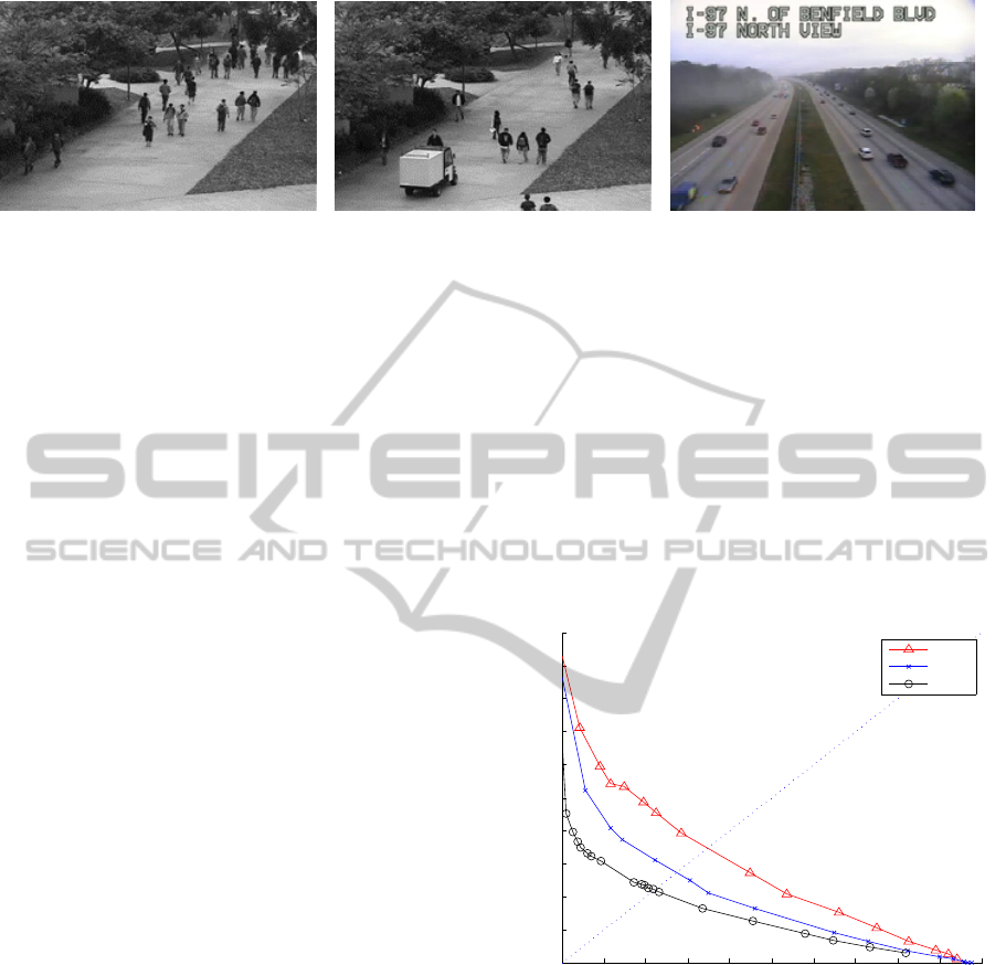
a) A representative training frame b) A representative testing frame c) A representative frame
in UCSD. with abnormality: golf car. from the direction dataset.
Figure 2: Representative frames from two datasets.
2008) is used, which is a public dataset for anormal-
ity detection. The UCSD dataset consists of two sub-
sets, Ped1 and Ped2, both having training and test-
ing parts. Classifiers are trained and testing frames
containing one or more abnormal features are defined
as abnormalities which are later compared with the
ground truth.
To detect direction abnormality, we obtain hours
of traffic cam footage from a highway in Maryland,
recorded from (mar, 2012). The refresh rate is 5fps
which is sufficient for optical flow given the motion
in the testset. To get more direction abnormalities,
we edit an hour long video sequence and reverse 15
small sections to simulate cars driving in the wrong
direction. The abnormalities are distributed randomly
over the entire video. The length of each sequence
spans from 25 frames (5 sec) to 125 frames (25 sec).
Representative frames in these two datasets are shown
in Figure 2.
3.2 Parameter Tuning
We first tune the texture parameters, then change the
threshold T
size
to find normalities and abnormalities
in the datasets. Similar to other works, we use False
Positive Rate (FPR) and False Negative Rate (FNR)
to quantify the results. From experimental investiga-
tions, the kernel size is set to approximately half of
the standard region size to get symmetric responses
on each side of the pixels. The radial frequency ω is
set to 2.3 and the frequency bandwidth K is set to π.
The only parameter that will be changed is the thresh-
old T
size
which regulates when a size is found to be
abnormal or not. The region size is set to 16 x 16
since the results are quite similar for all three optical
flow methods while varying the region size.
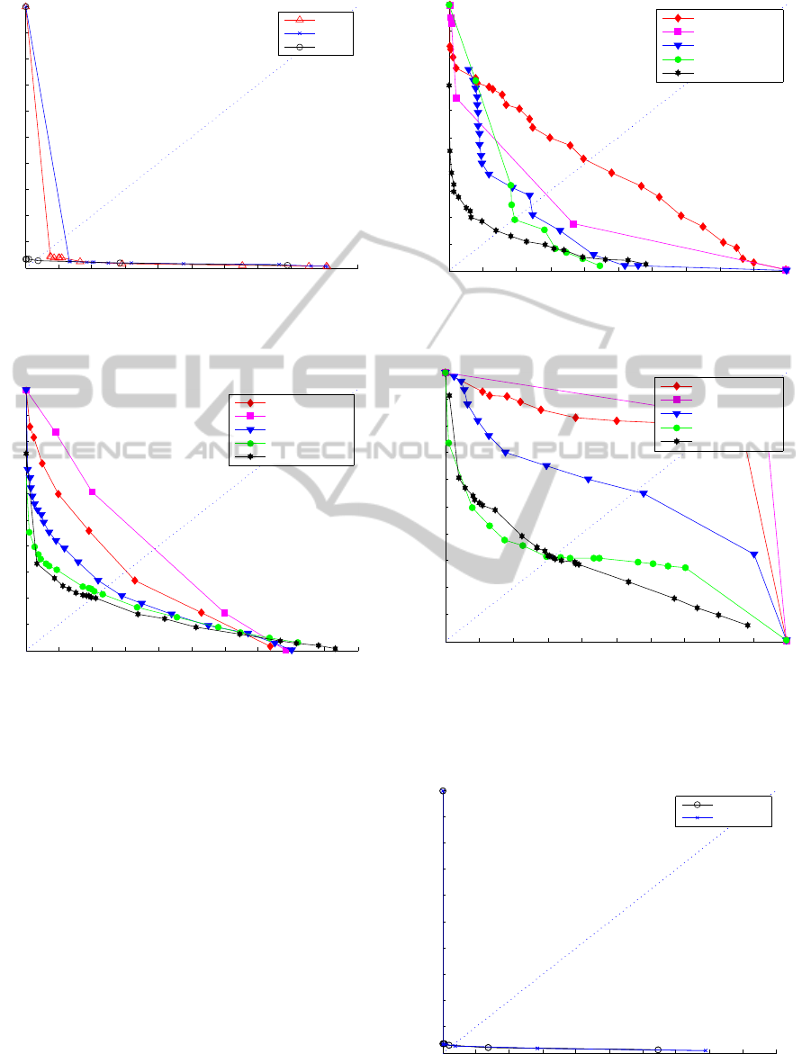
3.3 Choice of Optical Flow Method
The search window size for the optical flow is set to
15 x 15 pixels in the Lucas-Kanade based methods,
with three pyramid levels and 1000 foreground fea-
tures in Pyramid Lucas-Kanade. For Horn-Schunck
method the stop iteration criteria has been set to 20.
The three optical flow methods are tested with differ-
ent possible thresholds yielding the curves in figure 3
and 4 for the Ped1 and Directional datasets, respec-
tively. As can be seen, Pyramid Lucas-Kanade out-
performs the other two methods. This is primarily
due to the utilization of ”good features to track” that
finds structures with a high level of texture that in turn
reduces the aperture problem.
0 0.1 0.2 0.3 0.4 0.5 0.6 0.7 0.8 0.9 1
0
0.1
0.2
0.3
0.4
0.5
0.6
0.7
0.8
0.9
1
Frame−level anomaly detection on Ped1: optical flow algorithms
False Positive Rate
False Negative Rate
LK
HS
Pyr LK
Figure 3: Curve for Pyramid Lucas-Kanade, Lucas-Kanade
and Horn-Schunck at 20 histogram bins and region size of
16 x 16. Test dateset: Ped1.
3.4 Results
We test our system and compare the results with
other methods that test on the UCSD dataset. These
are: ”Reddy” (Reddy et al., 2011) , ”Social Force”
(Mehran et al., 2009) , ”MDT” (Mahadevan et al.,
2010) and ”MPPCA” (Kim and Grauman, 2009). The
results at frame level are shown in Figure 5 and 6.
Moreover we compare abnormality results at pixel
level, see Figure 7.
Real-timeMultipleAbnormalityDetectioninVideoData
393
0 0.1 0.2 0.3 0.4 0.5 0.6 0.7 0.8 0.9 1
0
0.1
0.2
0.3
0.4
0.5
0.6
0.7
0.8
0.9
1
Frame−level anomaly detection on direction dataset: optical flow algorithms.
False Positive Rate
False Negative Rate
LK
HS
Pyr LK
Figure 4: Curve for Pyramid Lucas-Kanade, Lucas-Kanade
and Horn-Schunck at 20 histogram bins and region size of
16 x 16. Test dateset: Directional.
0 0.1 0.2 0.3 0.4 0.5 0.6 0.7 0.8 0.9 1
0
0.1
0.2
0.3
0.4
0.5
0.6
0.7
0.8
0.9
1
Frame−level anomaly detection on Ped1
False Positive Rate
False Negative Rate
Social Force
MPPCA
MDT
Reddy
Proposed method
Figure 5: Frame level abnormality detection on Ped1.
We further calculate the Equal Error Rate (EER)
for frame level and pixel level abnormality detection,
respectively, see Table 1 and 2. It can be seen in
both the figures and tables that our method outper-
forms other methods in frame level abnormality and
for pixel level abnormality detection, the proposed
method performs as good as the best of the other
methods.
For the direction abnormalities we test on our own
dataset as explained above. The results are shown in
Figure 8 for two different strategies for direction vec-
tor updating. When computing the four dimensional
vector for direction feature, we can increase the direc-
tion bin by one or adding the gradient to the direction
bin, see results in Figure 8. The difference between
the single increment and the gradient increment of the
motion seems to be negligible. The total error rate is
0.3%.
At last, we show the computational requirements
0 0.1 0.2 0.3 0.4 0.5 0.6 0.7 0.8 0.9 1
0
0.1
0.2
0.3
0.4
0.5
0.6
0.7
0.8
0.9
1
Frame−level anomaly detection on Ped2
False Positive Rate
False Negative Rate
Social Force
MPPCA
MDT
Reddy
Proposed method
Figure 6: Frame level abnormality detection on Ped2.
0 0.1 0.2 0.3 0.4 0.5 0.6 0.7 0.8 0.9 1
0
0.1
0.2
0.3
0.4
0.5
0.6
0.7
0.8
0.9
1
Pixel−level anomaly detection on Ped1
False Positive Rate
False Negative Rate
Social Force
MPPCA
MDT
Reddy
Proposed method
Figure 7: Pixel level abnormality detection on Ped1.
for the different features. All tests are conducted on
an ASUS U46S with an Intel Core i5-2410M CPU
0 0.1 0.2 0.3 0.4 0.5 0.6 0.7 0.8 0.9 1
0
0.1
0.2
0.3
0.4
0.5
0.6
0.7
0.8
0.9
1
Frame−level anomaly detection on direction dataset: incrementing methods.
False Positive Rate
False Negative Rate
Add one
Add motion
Figure 8: Frame level abnormality detection on the direc-
tional dataset, with the two different updating methods.
VISAPP2013-InternationalConferenceonComputerVisionTheoryandApplications
394
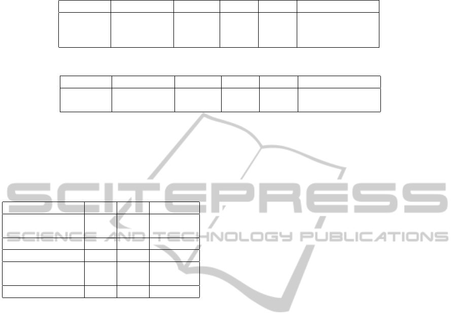
Table 1: EER for frame level abnormality detection on Ped1 and Ped2 subsets of UCSD.
Approach Social Force MPPCA MDT Reddy Proposed method
Ped1 31.0% 40.0% 25.0% 22.5% 20.0%
Ped2 42.0% 30.0% 25.0% 20.0% 15.0%
Average 37.0% 35.0% 25.0% 21.2% 17.5%
Table 2: EER for pixel level abnormality detection on Ped1 and Ped2 subsets of UCSD.
Approach Social Force MPPCA MDT Reddy Proposed method
Ped1 79.0% 82.0% 55.0% 32.0% 31.0%
Ped2 - - - - 21.0%
running at 2.30 GHz and are calculated with an aver-
age FPS in an entire test sequence run. As seen from
Table 3, the system is able to work even faster than
real-time.
Table 3: Datasets with their respective FPS using different
features.
Ped1 Ped2 Direction
Size 238 360 320
x158 x240 x240
Motion FPS 50 40 -
Size/Texture FPS 20 15
Motion & Size 18 12 -
/Texture FPS
Direction FPS 50
4 CONCLUSIONS
We propose a framework to detect multiple abnor-
malities in video surveillance, in which motion, size,
texture, with direction features are used to train inde-
pendent classifiers. Experiments show improvements
compared to related work. This result is partly caused
by less abnormalities in size and texture compared to
motion abnormalities in the datasets. Equally impor-
tantly, our proposed system is able to run faster than
real-time, which allows for connecting four or five
cameras to a single computer.
REFERENCES
(2008). Ucsd anomaly dataset. http://www.svcl.ucsd.edu/
projects/anomaly/dataset.html.
(2012). Maryland department of transportation. http://
www.traffic.md.gov/.
Boslaugh, S. and Watters, P. (2008). Statistics in a Nutshell.
O’Reilly Media, Inc.
Bouguet, J. (2000). Pyramidal implementation of the lucas
kanade feature tracker description of the algorithm.
Cui, X., Liu, Q., Gao, M., and Metaxas, D. (2011). Abnor-
mal detection using interaction energy potentials. In
CVPR.
Horn, B. and Schunck, B. (1981). Determining optical flow.
Artificial Intelligence.
Hu, W., Xiao, X., Fu, Z., Xie, D., Tan, T., and Maybank,
S. (2006). A system for learning statistical motion
patterns. PAMI.
Johnson, N. and Hogg, D. (1995). Learning the distribution
of object trajectories for event recognition. In British
conference on Machine vision.
Kim, J. and Grauman, K. (2009). Observe locally, infer
globally: A space-time mrf for detecting abnormal ac-
tivities with incremental updates. In CVPR.
Lee, T. (1996). Image representation using 2d gabor
wavelets. PAMI, 18:959–971.
Li, L., W. Huang, I. G., and Tian, Q. (2003). Foreground ob-
ject detection from videos containing complex back-
ground. In ACM international conference on Multi-
media.
Lucas, B. and Kanade, T. (1981). An iterative image regis-
tration technique with an application to stereo vision.
In International joint conference on Artificial intelli-
gence.
Mahadevan, V., Li, W., Bhalodia, V., and Vasconcelos, N.
(2010). Anomaly detection in crowded scenes. In
CVPR.
Mehran, R., Oyama, A., and Shah, M. (2009). Abnormal
crowd behavior detection using social force model. In
CVPR.
Piciarelli, C. and Foresti, G. L. (2006). On-line trajectory
clustering for anomalous events detection. Pattern
Recognition Letters, 27(15):1835–1842.
Reddy, V., Sanderson, C., and Lovell, B. (2011). Improved
anomaly detection in crowded scenes via cell-based
analysis foreground speed, size and texture. In Inter-
national Workshop on Machine Learning for Vision-
based Motion Analysis (CVPRW).
Stauffer, C. and Grimson, W. (2000). Learning patterns of
activity using real-time tracking. PAMI, 22(8):747–
757.
Yu, Q. and Medioni, G. (2009). Motion pattern interpre-
tation and detection for tracking moving vehicles in
airborne video. In CVPR.
Zhao, B., Li, F., and Xing, E. (2011). Online detection of
unusual events in videos via dynamic sparse coding.
In CVPR.
Real-timeMultipleAbnormalityDetectioninVideoData
395
