Segmentation of Crystal Defects via Local Analysis of Crystal Distortion

Matt Elsey and Benedikt Wirth

Courant Institute of Mathematical Sciences, New York University, 251 Mercer Street, New York, NY 10012, U.S.A.

Keywords:

Segmentation, Crystal Defect, Dislocation, Crystal Distortion, Variational Method, Sparse Curl.

Abstract:

We propose a variational method to simultaneously detect dislocations and grain boundaries in an image of

a crystal as well as the local crystal distortion. To this end we extract a distortion ﬁeld F from the image

which is nearly curl-free except at dislocations and grain boundaries. The sparsity of the curl is promoted by

an L

-regularization of curlF in the employed energy functional. The structure of the functional admits a fast

and parallelizable minimization such that fairly large images can be analyzed in a few minutes.

1 INTRODUCTION

Imagine we are given a large transmission electron

microscopy image or a simulated snapshot of a crys-

talline structure as in Fig. 1 left, and we want to de-

tect all crystal defects, statistically analyze the size

of defect-free regions, and evaluate correlations be-

tween crystal orientations in different regions, per-

haps even for a whole time sequence of such images.

Such tasks are of fundamental importance in materi-

als science and physics to better understand the be-

havior and properties of crystalline materials such as

metals, to validate mathematical models of such ma-

terials, to ﬁt model parameters, or even to optimize

material parameters. Often, the detection of crystal

defects and crystal orientation is accomplished man-

ually, e. g. (Wu and Voorhees, 2012), obviously with

limited feasibility for larger images or sets of data.

We here devise a new automatic crystal segmenta-

tion method which yields the crystal defects, the local

crystal orientation at each point, and the local crys-

tal strain and which can be computed efﬁciently via

a split Bregman iteration. The algorithm permits par-

allelization on a graphics processing unit (GPU) and

thereby allows for the automatic analysis of images of

a size as in Fig. 1 within few minutes.

We here restrict ourselves to two spatial dimen-

sions which is sufﬁcient for the classical application

of examining microscope images. A generalization to

three dimensions is straightforward.

The two subsequent sections provide the neces-

sary background on crystal structures and introduce

existing related methods before we present our model

and algorithm in Sec. 2 and 3 as well as some numer-

ical examples and a discussion in Sec. 4 and 5.

1.1 Grain Boundaries and Dislocations

We restrict our discussion to two dimensions. In a per-

fect atomic crystal, atoms are arranged in a Bravais

lattice: the atom positions are given by n

+ n

for two ﬁxed vectors a

∈ R

and all integers

. Real materials form polycrystals, that is, crys-

talline regions (so-called grains) of different orienta-

tions, meeting at grain boundaries (Fig. 2 left). These

grain boundaries are often denoted low or high angle

boundaries, depending on the orientation mismatch

between the adjacent grains.

Another type of crystal defect is a dislocation,

where a line of atoms terminates inside a crystal

(Fig. 2 middle). If we draw a closed curve (a so-

called Burgers circuit) on the perfect lattice and map

it onto the crystal around the dislocation (Fig. 2 right),

a gap remains whose direction and length deﬁne the

so-called Burgers vector.

Low angle grain boundaries are typically com-

posed of a sequence of dislocations (see e. g. Fig. 1).

Physicists are interested for instance in how de-

fects move and grain boundaries behave or in how the

grain size distribution evolves over time. To this end

crystal images are often analyzed manually.

1.2 Related Methods

Several efﬁcient approaches for the automatic analy-

sis of crystals do already exist, but they either only ap-

ply to molecular dynamics simulation results or they

only provide a segmentation into different grains but

ignore crystal strains or dislocations.

In (Berkels et al., 2008), the authors perform a

piecewise constant Mumford–Shah segmentation of a

294

Elsey M. and Wirth B..

Segmentation of Crystal Defects via Local Analysis of Crystal Distortion.

DOI: 10.5220/0004281502940302

In Proceedings of the International Conference on Computer Vision Theory and Applications (VISAPP-2013), pages 294-302

ISBN: 978-989-8565-47-1

 2013 SCITEPRESS (Science and Technology Publications, Lda.)

(

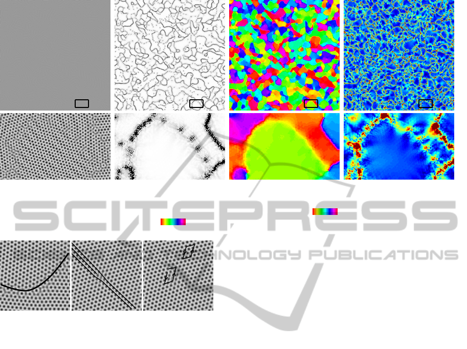
Figure 1: Given a crystal image (left), our method computes a distortion map F : Ω → R

2×2

whose curl magnitude indicates

crystal defects (second image; single spots are dislocations, dotted and continuous lines are low and high angle grain bound-

aries). Polar decomposition of F yields the local crystal orientation (third image, 0

π/3), and dist(F,SO(2)) can be

taken as a measure of crystal strain (right, 0 0.1).

Figure 2: Grain boundary between two grains (left), dislo-

cation with a terminating line of atoms (middle), and same

dislocation enclosed by a curve on the lattice which would

be closed away from the dislocation (right).

crystal image u : Ω → R into disjoint regions Ω

⊂ Ω

of constant crystal orientation α

∈ [0,2π), using a

Chan–Vese level set approximation. The model can

be augmented by a global deformation φ : Ω → R

de-

scribing the elastic crystal deformation in each region.

This approach involves a large number of nonlinearly

coupled degrees of freedom (the orientations α

, mul-

tiple level set functions, the deformation φ) and thus

is rather slow; also it concentrates on crystal grains

and ignores the structure of their boundaries or sin-

gle dislocations. Restricting to unstrained grains, the

authors in (Boerdgen et al., 2010) were able to give

a convex formulation of the above Mumford–Shah

segmentation problem based on functional lifting (in-

stead of using the orientation map α : Ω → [0,2π) one

rephrases the functional in terms of 1

: Ω × [0, 2π] →

[0,1], 1

(x,γ) = 1 if α(x) ≥ γ and 0 else). They also

propose a more efﬁcient version in which the inter-

faces between the Ω

are penalized according to the

local angle difference, a method which can be im-

proved further by taking into account the periodic-

ity of the angle (Strekalovskiy and Cremers, 2011).

A GPU implementation of this approach is fast, but

needs lots of memory due to the lifted variable 1

The method in (Singer and Singer, 2006) assumes

a rather clean crystal image with a perfectly regular,

unstrained grain interior. In that case the grain orien-

tation can be found very rapidly by ﬁrst convolving

with a wavelet resembling a grid cell and then locally

smoothing out the oscillatory pattern in the convolu-

tion. The resulting grey value indicates the average

mismatch between the crystal and the wavelet and can

thereby be identiﬁed with a crystal orientation. How-

ever, for slightly strained crystals this identiﬁcation is

erroneous; also one cannot distinguish between crys-

tal orientations which equally mismatch the wavelet.

The method seems to incidentally also identify dislo-

cations by a different gray value.

A fast, non-variational dislocation detection

method for three-dimensional molecular dynamics

data is proposed in (Stukowski and Albe, 2010a).

They ﬁrst identify perfectly crystalline regions by a

nearest neighbor analysis and then ﬁnd shortest Burg-

ers circuits around the non-perfect regions. This

yields the Burgers vector and location of all dislo-

cations. The method gains in robustness (but can

no longer be used on the ﬂy) by a technique of

sweeping out tubes around the dislocation lines in 3D

(Stukowski and Albe, 2010b). Additionally the au-

thors identify and triangulate grain boundaries which

are not composed of strings of dislocations. A simi-

larly efﬁcient method is introduced in (Begau et al.,

2012). Like our approach, it is based on identify-

ing the curl of the local crystal distortion, which in

a molecular dynamics simulation is readily obtained

from the positions of the nearest neighbor atoms.

In contrast to the above approaches, our method

SegmentationofCrystalDefectsviaLocalAnalysisofCrystalDistortion

295

simultaneously ﬁnds dislocations, grain boundaries,

and crystal distortion, just based on a crystal image.

2 VARIATIONAL MODEL

In this section we explain how to identify crystal

defects with curl concentrations of a distortion map

which arises from interpreting an imperfect crystal as

a deformed perfect crystal. We then introduce a sim-

ple energy functional whose minimization leads to the

detection of such curl concentrations.

2.1 Defects as Curl Concentrations

Imagine that a domain Ω ⊂ R

is occupied by a per-

fect, unstrained crystal without defects. If this crystal

is deformed according to a smooth deformation φ :

Ω → R

, which maps each position x inside the crys-

tal onto a new position φ(x), then the deformed crys-

tal is still defect-free, though it might be strained. A

polycrystal or a crystal with dislocations has a defect-

free, albeit strained, crystal structure away from grain

boundaries and dislocations. In those regions it can

thus be interpreted as a smoothly deformed perfect

crystal. Finding crystal defects hence amounts to the

identiﬁcation of places where such an interpretation

is not possible. How to accomplish this task?

In their variational approach (Berkels et al., 2008),

the authors attempt to directly ﬁnd the global defor-

mation φ together with a segmentation of the crys-

tal into different regions across whose boundaries φ

is discontinuous. These boundaries can then be in-

terpreted as grain boundaries, separating defect-free

crystal regions from each other. However, searching

a joint global segmentation and global deformation is

a highly nonlinear problem which makes the method

rather slow. Instead, it would be advantageous to

identify crystal defects based only on the local crystal

structure.

Assume, at each point x inside the crystal we know

the local crystal distortion, that is, the local amount

of rotation, stretching, and shearing (as compared to

an unstrained perfect crystal). This distortion can be

described by a linear map F(x) ∈ R

2×2

. In case of

a smoothly deformed perfect crystal, F : Ω → R

2×2

is given by the gradient of the crystal deformation φ,

F = ∇φ

= (∇φ

,∇φ

)

. In order to identify places

where the crystal cannot be described via a smooth

deformation of an unstrained perfect crystal, we now

have to ﬁnd those regions where F cannot be inter-

preted as the gradient of a deformation, that is, where

F is not conservative. It is well-known that a tensor

Figure 3: Photograph of a synthetic reptile skin (courtesy

http://www.stoff4you.de ) and detected regions of curl con-

centration encoded by color (inset), showing various dislo-

cations.

ﬁeld F is conservative if and only if it is curl-free,

curlF = (∂

− ∂

,∂

− ∂

) = 0.

The curl-free regions thus represent the defect-free in-

terior of crystal grains, while grain boundaries and

dislocations are characterized by nonzero curlF.

In particular, if the boundary between two grains

is sharp, F is simply discontinuous there and thus

has a measure-valued nonzero curl concentrated along

the boundary, while real crystals typically exhibit a

thin transition region across which the nonzero curl is

spread out. Likewise, the curl of F at a dislocation

behaves like a δ-peak. Its strength

curlF dx can be

computed via a line integral around the dislocation,

curlF(x)dx =

∂B

⊥

dx ,

where B is a ball around the dislocation and n

⊥

its

unit outward normal rotated counterclockwise by

The integrand describes how the curve ∂B is locally

stretched by the distortion F, and a nonzero integral

value shows that if one traces the distorted curve one

does not arrive at the starting point, but under- or over-

shoots according to the dislocation’s Burgers vector.

Indeed,

∂B

⊥

dx has the interpretation of the vector

spanning the gap in Fig. 2 right.

Fig. 3 shows the curl concentrations in the scales

pattern of a synthetic reptile skin. These are clearly

located in places where an additional row of scales

squeezes in between two rows. As discussed above,

the shown direction of the curl is related to the Burg-

ers vector and indicates the direction in which the ad-

ditional row of scales is inserted. A red dot for in-

stance implies that

∂B

⊥

dx points upwards, thus

there is vertical dilation left and compression right of

the dislocation so that additional scales are inserted

left of it.

VISAPP2013-InternationalConferenceonComputerVisionTheoryandApplications

296

2.2 Variational Curl Segmentation

Given an image u : Ω → R or some other measure-

ment of a crystal structure, we would like to extract

the distortion ﬁeld F : Ω → R

2×2

, which we expect

to have sparse curl, concentrated at dislocations and

grain boundaries.

We shall follow the usual paradigm in variational

image processing and devise an energy functional as

the sum of a ﬁdelity or ﬁtting term E

ﬁt

[F], which pe-

nalizes a mismatch between F and the given data u,

and a regularization term, which incorporates a priori

knowledge of the structure of F and correspondingly

regularizes F in the case of noisy input data. For regu-

larization we propose the L

(Ω)-norm of curlF since

the L

-norm is expected to promote sparseness. Thus

we arrive at an energy of the form

ﬁt

[F] + ω

kcurlFk

for some positive weight ω

. As for the ﬁtting term,

we restrict ourselves to images u as input data, in

which case we can use the term proposed in (Boerd-

gen et al., 2010),

ﬁt

[F] =

Ω

∑

(u(x + F(x)v

) − u(x))

dx , (1)

where v

,...,v

∈ R

represent a stencil of lattice

vectors such that in an image u of a perfect refer-

ence crystal we have u(x + v

) = u(x) for all x and

k = 1,. . . , K. The stencil elements v

can for instance

be chosen to agree with the K-fold rotational symme-

try of the crystal by

= `(cos(

2πk

),sin(

2πk

))

where ` represents the lattice spacing or characteristic

period of the input image. In the case of a hexagonal

crystal as in Fig. 1 we have K = 6.

Unfortunately, from an analytical viewpoint, the

regularization kcurlFk

in combination with a non-

convex ﬁtting term does not provide sufﬁcient com-

pactness to ensure existence of energy-minimizing

tensor ﬁelds F, even away from crystal defects, where

a classical minimizer would be expected. Also, exper-

imental results are improved by an additional smooth-

ing term so that for our crystal segmentation problem

we ﬁnally choose to minimize the energy

E[F] = E

ﬁt

[F] + ω

kcurlFk

+ ω

k∇Fk

(2)

with weights ω

,ω

> 0. For images with gray

values between 0 and 255, the choice (ω

,ω

) =

(4000`,8000`) seems to generally yield satisfactory

results.

3 MINIMIZATION ALGORITHM

Here we describe the algorithm used to segment im-

ages based on the energy (2). We begin by describ-

ing some of the properties of the model and make

the observation that we seek a local minimizer of (2).

For this reason, a good initial guess for F is required.

We propose one simple technique for initializing F.

Then we discuss the split Bregman formulation of

(Goldstein and Osher, 2009) for problems with L

type structure and indicate how we apply it to the pro-

posed segmentation model.

3.1 Initialization of F as Rotations

The ﬁtting term (1) makes the variational energy (2)

nonconvex. It can be readily seen that the global min-

imizer of (2), F ≡ 0, is not of interest. Instead, we are

interested in ﬁnding a local minimizer of (2) which is

close to an appropriately-chosen initial guess F

Two observations guide our choice of F

: The im-

ages of interest consist of large defect-free, perfectly

crystalline regions, and in those regions the local crys-

tal distortion can be very well described by a mere

rotation.

We choose F

(x) at each x ∈ Ω to be the rotation

matrix

(x) =



cos(α(x)) −sin(α(x))

sin(α(x)) cos(α(x))



=: R

α(x)

paramaterized by the angle α(x) which approximately

minimizes (1). To this end we consider a discrete

set of p angles, α

2π j

K p

with j = 0,. . . , p − 1.

At each pixel x we now identify that rotation R

which minimizes the integrand of (1) and either set

(x) = R

or F

(x) = R

∗

where α

∗

minimizes the

quadratic interpolation of

∑

(u(x + R

) − u(x))

α = α

,α

j±1

(the subscript ( j ± 1) is to be interpreted

mod p). In practice, we ﬁnd it sufﬁcient to choose

p ∼ 24/K.

3.2 L

-Type Minimization

The split Bregman formulation of (Goldstein and Os-

her, 2009) applies the Bregman iteration idea pro-

posed in (Bregman, 1967) and popularized by (Osher

et al., 2005) to a convex energy composed of both L

and L

-type terms. The idea is to introduce a new

variable ψ which corresponds to the L

-type term and

then to add the appropriate constraint term to enforce

this correspondence. Suppose E

[v] = kζ[v]k

+ H[v],

with both kζ[v]k

and H[v] convex. This approach ad-

vocates solving

min

v,ψ

kψk

+ H[v] subject to ζ[v] = ψ

SegmentationofCrystalDefectsviaLocalAnalysisofCrystalDistortion

297

via Bregman iteration, which is in this context given

k+1

,ψ

k+1

}=argmin

v,ψ

kψk

+H[v]+λkψ−ζ[v]−b

, (3)

k+1

= b

− ψ

k+1

+ ζ[v

k+1

]. (4)

The split Bregman simpliﬁcation is to perform alter-

nating minimization on v

k+1

and ψ

k+1

, which allows

for v

k+1

to depend only on L

-type terms, and gives

an explicit form for ψ

k+1

= argmin

H[v]+ λkψ

− ζ[v] − b

, (5)

k+1

= shrink(ζ[v

k+1

] + b

), (6)

k+1

= b

− ψ

k+1

+ ζ[v

k+1

], (7)

with

shrink(z,ω) :=

|z|

max(|z| − ω,0).

Theorems proven in (Osher et al., 2005) and

(Goldstein and Osher, 2009) guarantee that if the min-

imization problem (3) can be solved exactly, a mini-

mizer of kψk

+H[v] is found which satisﬁes the con-

straint ψ = ζ[v], i. e. one which solves the original

minimization problem. The split Bregman simpliﬁ-

cation suggests that a single alternating minimization

step for v

k+1

and ψ

k+1

is taken to approximate (3),

however very good results and fast convergence are

still observed in practice. The advantage is that the

original energy, which had both L

- and L

-character,

has now been reduced to a standard convex L

mini-

mization problem to advance v and to a pointwise and

explicitly known update in the new variable ψ.

The minimization problem considered here does

not satisfy the hypothesis of the theorem, as E

ﬁt

[F]

is nonconvex, but the Bregman scheme appears to be

very successful at locating a local minimum of our

energy anyhow. We set

H[F] = E

ﬁt

[F] + ω

k∇Fk

ζ[F] = ω

curl(F)

and apply the update (5)–(7).

In order to perform the update (5), we apply the

Fletcher–Reeves nonlinear conjugate gradient method

with Armijo stepsize control, as Hessian-based meth-

ods are not expected to (and in practice do not) pro-

vide much beneﬁt for the nonconvex ﬁtting energy E

ﬁt

which also requires interpolation of the image u. We

employed biquadratic interpolation which does not in

general guarantee a continuous interpolation, much

less one which is continuously twice differentiable.

4 NUMERICAL EXPERIMENTS

Fig. 1 already showed a result of our method, applied

to a snapshot from a phase ﬁeld crystal simulation

Figure 4: Original image and algorithm output for an ini-

tialization of F with rotations in [0,π/3) (left) and rotations

in [π/6,π/2) (right). The top row shows the crystal orien-

tation (0 π/2, obtained via polar decomposition), the

bottom row shows |curlF|. The interpretation of the bottom

left grain as being oriented at 0 rather than the equivalent

π/3 leads to spurious curl.

(PFC, see e. g. (Elder and Grant, 2004)) with hexago-

nal crystals. Our method provides the crystal distor-

tion ﬁeld F at each pixel from which useful and intu-

itive output can readily be derived: The locations of

high |curlF| represent crystal defects (either disloca-

tions or grain boundaries, second image in Fig. 1), the

rotation R of a polar decomposition F = HR (where

H ∈ R

2×2

is symmetric and R ∈ SO(2)) reveals the

local crystal orientation and thus the extent of crystal

grains (third image), and the distance of F to SO(2)

has the interpretation of an elastic strain (right image).

Together, these pieces of information fully describe

the mesoscopic state of the polycrystal.

In the following sections we provide more exam-

ples of how to deal with large polycrystal images or

crystals of different symmetries, and we report the

typical computational effort.

4.1 Accounting for Point Groups

Especially in images of polycrystals there still re-

mains an issue with the interpretation of our results:

Any two matrices F

should actually be interpreted

as equivalent if they only differ by the point group

P of the crystal (the set of all rotations and reﬂec-

tions that leave {v

,...,v

} invariant). Indeed, if

= F

P for a P ∈ P, then the crystal distorted by

looks identical to the one distorted by F

. Our

model does not automatically account for that fact

and interprets F

and F

as different distortions, which

can lead to spurious curl accumulations as shown in

Fig. 4. As a remedy, we once initialize F with ro-

tations between [0,

2π

) and once with rotations be-

tween [

3π

). The result F

from the ﬁrst initializa-

tion typically shows spurious curl along boundaries

of grains at an orientation close to 0 or

2π

, while the

second result, F

, does so at grain orientations around

and

3π

. We now simply identify regions of spuri-

VISAPP2013-InternationalConferenceonComputerVisionTheoryandApplications

298

Figure 5: After smoothing out the curl of both results in

Fig. 4 (left, middle) we identify the region where the ﬁrst

has higher values (blue region in right image). In this region

we replace the ﬁrst output by the second output, yielding the

shown curl (right).

ous curl by comparing |curlF| in both results: in re-

gions where F

has a signiﬁcantly higher curl than F

we use F

instead of F

. In detail, we ﬁrst smooth

|curlF

| and |curlF

| (e. g. convolving with a Gaussian

G of roughly two unit cell widths), then we pick the

region where G ∗ |curlF

| − G ∗ |curlF

| lies above a

certain small threshold (in our simulations 0.01) and

dilate this region by two unit cells. Within this region

we consider F

as the correct distortion, outside F

(Fig. 5).

4.2 Coarsening Simulations

As a demonstration of this method, we segment a time

series of crystals chosen from a PFC evolution. In

Fig. 6, four time snapshots of the PFC evolution are

considered (left to right). The resulting rotation map,

local volume distortion map (measured as det F − 1),

elastic strain map, and curl magnitude map are dis-

played for each time point (top to bottom). Though

each segmentation is performed independently, it can

be seen that rotations are assigned in a consistent way.

Volume distortion and strain are nonzero near grain

boundaries and dislocations. High magnitude of curl

(|curlF|) is seen to denote grain boundaries and iso-

lated dislocations, which can be easily distinguished

from each other. Note that each dislocation creates a

dipole structure in the volume distortion map, since

the crystal is dilated on one side of the dislocation

and compressed on the other. The orientation of this

dipole can hence also be used as an indicator of the

Burgers vector.

4.3 Strained Crystals

In contrast to the approaches from Sec. 1.2, our

method directly provides the crystal strain, which can

be of interest in particular for the analysis of non-

equilibrated crystals. As a simple example, we per-

formed a PFC simulation, where in regular time inter-

vals we artiﬁcially shift a stripe of the simulated ma-

terial horizontally by one pixel, thereby emulating the

effect of a shearing force. The resulting strained crys-

tals are shown in Fig. 7, once for a defect-free crystal

and once for a crystal with three dislocations. The

distribution of elastic strains indicates that the dislo-

cations effectively reduce the strain in the bulk of the

material (while there is a higher peak strain in close

vicinity to the crystal defects).

4.4 Different Crystal Types

The method seems to work robustly on different types

of input images, including real experimental images.

Fig. 8 shows a HRTEM image of a nanocrystalline

palladium thin ﬁlm, courtesy of Nick Schryvers, from

the work (Wang et al., 2012). The tensor ﬁeld F is

robustly extracted, even though the coloring varies

across the image, and |curlF| correctly identiﬁes an

isolated dislocation. The crystalline orientation ob-

tained from polar decomposition of F reveals that

three distinct regions separated by twin boundaries

are identiﬁed correctly despite no more than 10

◦

dif-

ference in orientation.

In Fig. 3 we used an even more challenging input

image of a reptile skin, whose pattern is rather irreg-

ular compared to an atomic crystal. Nevertheless, us-

ing the six-point stencil of hexagonal symmetry, the

locations as well as the types of the dislocations in

the scales pattern are correctly identiﬁed. Note that

the unit cells of the pattern vary strongly in size so

that our initialization of F with pure rotations seems

much less appropriate, yet it obviously still sufﬁces to

achieve the desired local minimizer.

Lattices of different than six-fold rotational sym-

metry can be analyzed using an appropriately adapted

stencil v

,...,v

. Fig. 9 shows a snapshot of a PFC

simulation with cubic lattice symmetry, for which

an appropriate stencil is given by v

= (`,0)

, v

(0,`)

, v

= (−`,0)

, v

= (0,−`)

(where again,

` is the characteristic spacing). The underlying PFC

model is a modiﬁcation of the standard PFC model,

presented in (Wu et al., 2010, Sec. VI) and originally

proposed in (Lifshitz and Petrich, 1997) in the context

of the Swift–Hohenberg equation. Isolated disloca-

tions as well as low- and high-angle grain boundaries

are properly identiﬁed. The local crystal orientation

indicates that most grains have similar orientations,

with atoms that in this particular simulation tend to

align well with the computational grid.

4.5 Computational Effort

For images as in Fig. 1 we generally found twenty

split Bregman steps to be sufﬁcient, in each of which

we perform ﬁve nonlinear conjugate gradient steps

SegmentationofCrystalDefectsviaLocalAnalysisofCrystalDistortion

299

Figure 6: Results of our algorithm applied to different snapshots of a phase ﬁeld crystal (PFC) coarsening simulation. From

top to bottom we show the time evolution of local crystal orientation (0 π/3), local volume distortion of the crystal

measured as detF − 1 (−0.05 0.05), elastic strain measured as dist(F,SO(2)) (0 0.05), and |curlF|.

0.0 0.5 1.0

Figure 7: PFC simulation of a sheared crystal without (top) and with (bottom) defects, showing the crystal image (left), the

elastic strain dist(F,SO(2)) (middle, 0 0.15), and F

(right, −0.2 0.2). The rightmost graph shows a histogram

of dist(F, SO(2)). The crystal with defects has a higher peak strain, but lower overall strain.

VISAPP2013-InternationalConferenceonComputerVisionTheoryandApplications

300

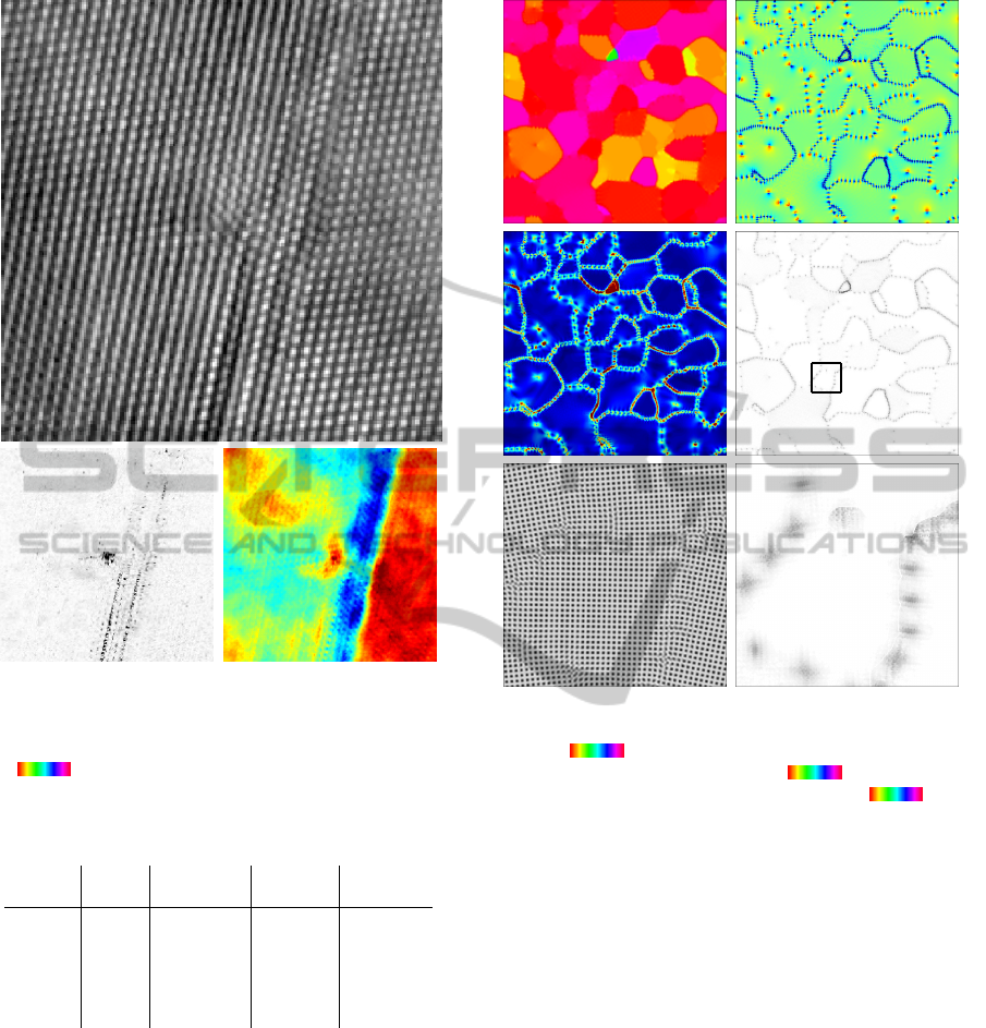
Figure 8: HRTEM image of a nanocrystalline palladium

thin ﬁlm, from (Wang et al., 2012), detected regions of

curl concentration showing an isolated dislocation, and

the crystal orientation obtained from polar decomposition

◦

) showing two twin boundaries.

Table 1: Rounded computation times of GPU implementa-

tion in Matlab for image in Fig. 1 and segments thereof.

image total split NCG inter-

size time Bregman descent polation

2048

380 s 312 s 296 s 160 s

1024

140 s 108 s 104 s 56 s

512

88 s 66 s 62 s 34 s

256

68 s 48 s 46 s 26 s

128

58 s 40 s 38 s 20 s

for (5). The code is implemented in Matlab, using

the included basic GPU support. Computation times

on a Tesla S10 GPU are displayed in Tab. 1 for dif-

ferent image sizes. For an image with 2048

pix-

els, the minimization takes slightly above six minutes

of which the net time inside the split Bregman iter-

ation (without screen output of the energy values) is

roughly 82%. Most of the iteration time is spent in

the nonlinear conjugate gradient steps which in turn

spend more than half of their time interpolating the

image u to evaluate the ﬁtting energy and its gradient.

We observe a strongly sublinear scaling with image

size due to the high GPU parallelization.



Figure 9: Results of our algorithm applied to microstruc-

ture with cubic symmetry. We show the local crystal orien-

tation (0 π/2, top left), local volume distortion of the

crystal measured as det F −1 (−0.05

0.05, top right),

elastic strain measured as dist(F,SO(2)) (0 0.05,

middle left), |curlF| (middle right), a zoom-in on the mi-

crostructure (bottom left), and a zoom in on |curlF| (bottom

right).

The bottleneck seems to lie in the evaluation of

u(x + F(x)v

) at each pixel x and for each stencil vec-

tor v

(computation times are reported for a six-point

stencil). This image interpolation requires almost un-

structured memory access which without code opti-

mization is not very efﬁcient on a GPU. Nevertheless

a speedup can be expected from a non-Matlab imple-

mentation tailored to the GPU architecture.

5 DISCUSSION

The proposed model is an efﬁcient tool for the

mesoscale analysis of polycrystals, an important task

in materials science. It can analyze fairly large images

in reasonable time, providing information about de-

fect locations and local crystal distortion, from which

different types of statistical data can readily be de-

SegmentationofCrystalDefectsviaLocalAnalysisofCrystalDistortion

301

rived. However, the simple Matlab implementation is

limited in its applicability to image sizes up to around

2000

pixels, which can resolve roughly 5·10

atoms.

With a tailored GPU implementation, this limit could

probably be pushed back considerably.

Note that in some cases simpler methods are avail-

able. If the atom positions do not have to be ex-

tracted from images, but are known for instance from

a molecular dynamics simulation, then the faster non-

variational methods from Sec. 1.2 can be employed.

The advantage of our approach over these methods

lies in the higher generality of the input data. Also,

for images from phase ﬁeld crystal (PFC) simula-

tions, the PFC energy density already identiﬁes de-

fect locations (but not the local distortion) quite well

for a range of model parameters. Furthermore, even

though the local crystal orientation does indicate grain

regions and can easily be obtained from our results,

our method does not provide a sharp image segmen-

tation into grains. The segmentation methods from

Sec. 1.2 are better suited for such a purpose, however,

they necessarily ignore single dislocations and details

of the grain boundary structure. Overall, our method

robustly yields more detailed and versatile informa-

tion of the mesoscopic crystal structure (such as local

strain or dislocation character) than previously exist-

ing methods, and it does so much faster than methods

that try to extract a slightly lower level of detail from

similarly general input data.

Finally, let us mention that our model is noncon-

vex and thus requires a sufﬁciently good initialization

before minimization (which can be obtained at low

cost in most cases). Also, the nonconvexity implies

that the analytical convergence results for the split

Bregman method cannot be relied on. Furthermore,

a better mathematical understanding of the mutual in-

ﬂuence and relative importance between the curl reg-

ularization and the smoothing of the distortion ﬁeld

might help to further improve the algorithm.

ACKNOWLEDGEMENTS

The authors thank Bob Kohn for continual advice and

suggestions throughout the preparation of this work.

ME and BW gratefully acknowledge the support of

NSF grant OISE–0967140 and a Courant Instructor-

ship, respectively.

REFERENCES

Begau, C., Hua, J., and Hartmaier, A. (2012). A novel ap-

proach to study dislocation density tensors and lattice

rotation patterns in atomistic simulations. Journal of

the Mechanics and Physics of Solids, 60(4):711–722.

Berkels, B., R

atz, A., Rumpf, M., and Voigt, A. (2008). Ex-

tracting grain boundaries and macroscopic deforma-

tions from images on atomic scale. J. Sci. Comput.,

35(1):1–23.

Boerdgen, M., Berkels, B., Rumpf, M., and Cremers, D.

(2010). Convex relaxation for grain segmentation at

atomic scale. In Fellner, D., editor, VMV 2010 - Vi-

sion, Modeling & Visualization, pages 179–186. Eu-

rographics Association.

Bregman, L. M. (1967). The relaxation method of ﬁnding

the common point of convex sets and its application

to the solution of problems in convex programming.

USSR Comput. Math. Math. Phys., 7(2):200–217.

Elder, K. R. and Grant, M. (2004). Modeling elastic and

plastic deformations in nonequilibrium processing us-

ing phase ﬁeld crystals. Phys. Rev. E, 70:051605.

Goldstein, T. and Osher, S. (2009). The split Bregman

method for L1–regularized problems. SIAM J. Imag.

Sci., 2(2):323–343.

Lifshitz, R. and Petrich, D. M. (1997). Theoretical model

for Faraday waves with multiple-frequency forcing.

Phys. Rev. Lett., 79(7):1261–1264.

Osher, S., Burger, M., Goldfarb, D., Xu, J., and Yin, W.

(2005). An iterative regularization method for total

variation-based image restoration. Multiscale Model.

Simul., 4(2):460–489.

Singer, H. M. and Singer, I. (2006). Analysis and visu-

alization of multiply oriented lattice structures by a

two-dimensional continuous wavelet transform. Phys.

Rev. E, 74:031103.

Strekalovskiy, E. and Cremers, D. (2011). Total varia-

tion for cyclic structures: Convex relaxation and ef-

ﬁcient minimization. In Computer Vision and Pat-

tern Recognition (CVPR), 2011 IEEE Conference on,

pages 1905–1911.

Stukowski, A. and Albe, K. (2010a). Dislocation detec-

tion algorithm for atomistic simulations. Modelling

and Simulation in Materials Science and Engineering,

18(2):025016.

Stukowski, A. and Albe, K. (2010b). Extracting disloca-

tions and non-dislocation crystal defects from atom-

istic simulation data. Modelling and Simulation in

Materials Science and Engineering, 18(8):085001.

Wang, B., Idrissi, H., Galceran, M., Colla, M., Turner,

S., Hui, S., Raskin, J., Pardoen, T., Godet, S., and

Schryvers, D. (2012). Advanced TEM investigation

of the plasticity mechanisms in nancrystalline free-

standing palladium ﬁlms with nanoscale twins. Int.

J. Plast., 37:140–156.

Wu, K.-A., Adland, A., and Karma, A. (2010). Phase-

ﬁeld-crystal model for fcc ordering. Phys. Rev. E,

81:061601.

Wu, K.-A. and Voorhees, P. W. (2012). Phase ﬁeld crys-

tal simulations of nanocrystalline grain growth in two

dimensions. Acta Materialia, 60(1):407–419.

VISAPP2013-InternationalConferenceonComputerVisionTheoryandApplications

302