
OpenOF
Framework for Sparse Non-linear Least Squares Optimization on a GPU
Cornelius Wefelscheid and Olaf Hellwich
Computer Vision and Remote Sensing, Berlin University of Technology,
Sekr. MAR 6-5, Marchstrasse 23, D-10587, Berlin, Germany
Keywords:
Least Squares Optimization, Bundle Adjustment, Levenberg Marquardt, GPU, Open Source.
Abstract:
In the area of computer vision and robotics non-linear optimization methods have become an important tool.
For instance, all structure from motion approaches apply optimizations such as bundle adjustment (BA). Most
often, the structure of the problem is sparse regarding the functional relations of parameters and measurements.
The sparsity of the system has to be modeled within the optimization in order to achieve good performance.
With OpenOF, a framework is presented, which enables developers to design sparse optimizations regarding
parameters and measurements and utilize the parallel power of a GPU. We demonstrate the universality of our
framework using BA as example. The performance and accuracy is compared to published implementations
for synthetic and real world data.
1 INTRODUCTION
Non-linear least squares optimization is used in many
research fields where measurements with an under-
lying model are present. Most of the problems con-
sist of hundreds of measurements and are represented
by hundreds of parameters that need to be estimated.
Minimizing the L2-norm between the actual measure-
ment and the estimated value is established by e.g.
solving a least squares system. Usually, as the un-
derlying model is not linear, an iterative method for
solving non-linear least squares needs to be applied.
Such methods linearize the cost function in each it-
eration. The Levenberg-Marquardt (LM) algorithm
has more or less become a standard. It combines
the Gauss-Newton algorithm with the gradient de-
scent approach. In contrast to other approaches, LM
guarantees convergence. The computationally most
intensive part within LM is solving Ax = b in each
iteration. Finding the solution of this normal equa-
tion for a dense matrix has a complexity of O(n
3
).
This is not effective when dealing with 100k - 1M
parameters on a standard computer. As most of the
entries in A are zero, a sparse matrix representation
is feasible. Different parametrization for sparse ma-
trices have been used in the past. Most commonly a
coordinate list (COO) is used, which stores for each
entry row, column and value. A more compact stor-
age is represented by the compressed sparse column
(CSC) format. For each entry, the row and the value
are stored in an array. Additionally, the starting in-
dex of each column is saved separately, requiring less
space than COO. The reduction of space between
COO and CSC is neglectable, while the implemen-
tation of efficient algorithms for matrix-vector multi-
plications is important. Since the operations on ma-
trices can be implemented in a highly parallel man-
ner, we believe that multiprocessors, such as GPUs,
are most suitable for this task. The operations within
LM are as well highly parallel, as each cost function
can be evaluated independently. To our knowledge
no library has been developed which can solve gen-
eral sparse non-linear least squares optimizations on
a GPU. Two libraries address this problem in general,
sparseLM (Lourakis, 2010) and g2o (Kummerle et al.,
2011), both operating on a CPU. For solving the nor-
mal equation, they implemented interfaces to various
external sparse math libraries, which provide differ-
ent algorithms for direct solving the normal equation.
In most cases a Cholesky decomposition A = LDL
T
is applied. In contrast to sparseLM, our approach
works on a GPU (presently only NVIDIA graphics
cards are supported) and uses the high parallel power
of the graphics card to solve the normal equation with
a conjugate gradient (CG) approach, which can also
be chosen as a solver in g2o. The potential of paral-
lelizing CG is the main advantage over a Cholesky
decomposition. Our framework is built upon three
260
Wefelscheid C. and Hellwich O..
OpenOF - Framework for Sparse Non-linear Least Squares Optimization on a GPU.
DOI: 10.5220/0004282702600267
In Proceedings of the International Conference on Computer Vision Theory and Applications (VISAPP-2013), pages 260-267
ISBN: 978-989-8565-48-8
Copyright
c
2013 SCITEPRESS (Science and Technology Publications, Lda.)

major libraries, Thrust, CUSP and SymPy. Thrust
enhances the productivity of developers by providing
high level interfaces for massive parallel operations
on multiprocessors. Thrust is integrated in the current
CUDA version 4.2 and supported by NVIDIA. The
framework presented in this paper can directly take
advantage of any improvements. The library CUSP
is based on Thrust and provides developers with rou-
tines for sparse linear algebra. The library SymPy is
an open source library for symbolic mathematics in
Python. The aim of our work is to give scientists a
new tool to test new models in less amount of time.
Using SymPy in our framework enables us to define
least squares models within a high level scripting lan-
guage. Starting from this, our framework automati-
cally generates C++ code which is compiled, gener-
ating the OpenOF optimization library, which can ei-
ther be called from C++ programmes for efficient use,
or from Python for rapid prototyping. OpenOF will
be published as open source library under the GNU
GPL v3 license.
2 RELATED WORK
Recently, non-linear optimization has gathered a lot
of attention. It has been successfully applied in dif-
ferent areas, e.g. Simultaneous Localization and Map-
ping (SLAM) or BA. We will use BA for evaluating
our framework, as it is a perfect example for a rather
complex but sparse system. Several libraries can be
used to solve BA. The SBA library (Lourakis and Ar-
gyros, 2009) which is used by several research groups
takes advantage of the special structure of the Hessian
matrix to apply the Schur complement for solving the
linear system. Nevertheless it has several drawbacks.
Integrating additional parameters which remain iden-
tical for all measurements (e.g. camera calibration) is
not possible, as the structure would change such that
the Schur complement could not be applied anymore.
With OpenOF, we provide a solution for those prob-
lems.
sparseLM (Lourakis, 2010) provides a software
package which is supposed to be general enough to
handle the same kind of problems as OpenOF does.
However, integrating new models within sparseLM is
time consuming. The performance is slow for prob-
lems with many parameters, as no multithreading is
integrated.
More recently another framework was developed
for similar purposes in graph optimization (Kum-
merle et al., 2011). In g2o, the Jacobian is evaluated
by numerical differentiation which is time consuming
and also degrades the convergence rate. Developers
can choose between direct (Davis, 2006) and itera-
tive solver such as CG. Kummerle et al. (2011) claims
that CG is most often slower than a direct solver. In
our experience direct solvers are more precise. How-
ever utilizing the parallelism of multiprocessors, CG
can be significantly faster. Applying a preconditioner
to CG has a large impact on the speed of conver-
gence. g2o uses a block Jacobi preconditioner. For
simplicity we use a diagonal preconditioner which has
been applied successfully for various tasks. A big
advantage of the diagonal preconditioner is, that the
least squares CG is computed directly from the Ja-
cobian without explicitly calculating the Hessian ma-
trix. Several other approaches (Kaess et al., 2011),
which address only a subset of problems, have been
presented previously for least squares optimization.
But so far no library provides the speed, the ease of
use and the generality to become a milestone within
the communities of computer vision or robotics.
3 LEVENBERG-MARQUARDT
LM is regarded as standard for solving non-linear
least squares optimization. It is an iterative approach
which was first developed by Levenberg in 1944 and
rediscovered by Marquardt in 1963. The algorithm
determines the local minimum of the sum of least
squares of a multivariant function. An overview of the
family of non-linear least squares optimization tech-
niques can be found in (Madsen et al., 2004). LM
combines a Gauss-Newton method with a steepest de-
scent approach. Given a parameter vector x we want
to find a vector x
min
that minimizes the function g(x)
which is defined as the sum of squares of the vector
function f (x).
x
min
= argmin
x
g(x) = argmin
x
1
2
m
∑
i=0
f
i
(x)
2
(1)
As the function is usually not convex, a suitable initial
solution x
0
needs to be provided. Otherwise, LM will
not converge to the global optimum, but get stuck in
a local minimum, which might be far away from the
optimal solution. In each iteration i, g(x) is approxi-
mated by a second order Tailor series expansion.
˜g(x) = g(x
i
) + g(x
i
)
0
(x − x
i
) +
1
2
g(x
i
)
00
(x − x
i
)
2
(2)
To find the minimum the first derivative of Equation
2 is set to zero, resulting in
∂ ˜g(x)
∂x
= g(x
i
)
0
+ g(x
i
)
00
(x − x
i
) = 0 . (3)
The first order derivative at the point x
i
can be re-
placed by the transposed Jacobian J
T
multiplied with
OpenOF-FrameworkforSparseNon-linearLeastSquaresOptimizationonaGPU
261

the residual. The second order derivative is approxi-
mated by the Hessian matrix given as J
T
J. The pa-
rameter update h = x −x
i
in each iteration is acquired
by solving the normal equation.
J
T
Jh = −J
T
f (x
i
) (4)
To include the gradient descent approach, Equation 4
is extended by a damping factor µ. For µ → 0 LM
applies the Gauss-Newton method and for µ → ∞ a
gradient descent step is executed.
(J
T
J + µI)h = −J
T
f (x
i
) (5)
If the update step does not result in a smaller error the
damping factor is increased pushing the parameters
further towards the steepest descent. Else, the update
is performed and the damping factor is reduced. In
cases with a known covariance of the measurements,
Equation 5 is extended to
(J
T
Σ
−1
J + µI)h = −J
T
Σ
−1
f (x
i
) . (6)
Instead of the Euclidean norm the Mahalanobis dis-
tance is minimized. Solving the normal equation is
the most demanding part of the algorithm. If the nor-
mal matrix has a certain structure, approaches such
as the Schur complement can be applied. Generally,
the normal equation can be solved with a Cholesky
decomposition. Another alternative is an iterative ap-
proach such as CG, which is incorporated in OpenOF.
In the next section, the CG approach will be described
in more detail.
4 CONJUGATE GRADIENT
The CG method is a numerical algorithm for solving
a linear equation system Ax = b with A being sym-
metric positive definite and x, b ∈ R
n
. As CG is an
iterative algorithm, there exists a residual vector r
k
in
each step k defined as:
r
k
= Ax
k
− b . (7)
CG belongs to the Krylov subspace methods. Krylov
subspace is described by
K
k
(A, r
0
) = span{r
0
, Ar
0
, A
2
r
0
, .. . , A
k−1
r
0
} . (8)
It is the basis for many iterative algorithms. There
is proof that those methods terminate in at most n
steps. CG is a highly economical method which does
not require much memory or time demanding matrix-
matrix multiplication. While applying CG, a set of
conjugate vectors (p
0
, p
1
, ..,p
k−1
, p
k
) is computed be-
longing to the Krylov subspace. In each step the al-
gorithm computes a vector p
k
being conjugate to all
previous vectors. A great advantage is that only the
previous vector p
k−1
is needed. Thus, the other vec-
tors can be omitted, thereby saving memory. The al-
gorithm is based on the principle that p
k
minimizes
the residual over one spanning direction in every it-
eration. CG is initialized with r
0
= Ax
0
− b, p
0
=
−r
0
, k = 0. In each iteration a step length α is com-
puted, which minimizes the residual over the current
spanning vector p
k
.
α
k
= −
r
T
k
r
k
p
T
k
Ap
k
(9)
The update of the current approximate solution is
given by
x
k+1
= x
k
+ α
k
p
k
(10)
which results in a new residual
r
k+1
= r
k
+ α
k
Ap
k
. (11)
The new conjugate direction is computed from Equa-
tions 12 and 13.
β
k+1
= −
r
T
k+1
r
k+1
r
T
k
r
k
(12)
p
k+1
= r
k+1
+ β
k+1
p
k
(13)
Finally k is increased. This procedure is repeated as
long as ||r
k
|| > ε and k < k
max
. In most cases, only
a few iterations are necessary as the CG method is
used within the iterative LM algorithm. For prove of
convergence and full derivation we refer to (Nocedal
and Wright, 1999).
For practical considerations the explicit computa-
tion of the matrix A = J
T
J can be omitted. Concate-
nating matrix-vector multiplications for J
T
and J is
faster and the numerical precision is higher. Such an
approach is known as least squares CG.
5 FRAMEWORK
OpenOF aims at making development cycles faster. It
saves the time of the developer searching for errors by
automatic code generation, but not at the expense of
computational efficiency. As we use fast high level
libraries on a GPU, the generated executable gains
performance. The design of the underlying model
assumes different types of objects containing groups
of parameters.These objects are linked by measure-
ments. The objects can be combined in arbitrary ways
(see Fig. 1). Usually, the computation of the Jacobi
matrix is either done by hand, or with the help of a
symbolic toolbox (SymPy, Matlab). Both cases are
error prone. The mistakes easily occure when ei-
ther transferring the code into an optimization library
VISAPP2013-InternationalConferenceonComputerVisionTheoryandApplications
262

Opt. Obj. Type 1 Opt. Obj. Type 3Opt. Obj. Type 2
Meas. Type 1 Meas. Type 2
Figure 1: Optimization objects interact with different mea-
surement types.
such as sparseLM (Lourakis, 2010) or from generat-
ing the derivatives by hand. This step needs to be done
each time small changes are made in the underlying
model. As the cost function usually can be described
in various ways, exploring which modeling of e.g. re-
lations between unknowns and measurements works
best is time consuming. Additionally the convergence
rate highly depends on the chosen model e.g. a con-
vex cost function is most preferable. In OpenOF the
model can be adjusted without further low level pro-
gramming steps, as the necessary code is generated
automatically. The main optimization is designed in
a modular way, enabling developers to easily mod-
ify the optimization algorithm or add new algorithms
while still having the advantage of the high perfor-
mance of a GPU.
An optimization task often comprises thousands
of parameters. Usually several entities have the same
meaning, e.g. (x, y) refer to the coordinate of a point.
Furthermore, these parameters can be grouped to ob-
jects. Within OpenOF all parameters are assigned to
an object. When designing optimization objects, we
distinguish between two different kinds of parame-
ters:
• Variable parameters
• Fixed parameters
The variable parameters will be adjusted within the
optimization. The fixed parameters remain constant
but are necessary to evaluate the cost function. Most
often we end up with a small number of different
types of objects. These objects are linked by so
called measurement types. A measurement represents
a function on which the least squares optimization is
performed. The user defines the function representing
relations between the different objects. Usually, not
all types of objects are necessary to evaluate a certain
measurement (see Figure 1). Sometimes we have a di-
rect but noisy observation X
obs
, e.g. the position given
from a GPS sensor. In this case we define a mea-
surement f (X
est
, X
obs
) = X
est
− X
obs
. It is clear that
the observation X
obs
is not allowed to change. This
function can be modeled in two ways in OpenOF. For
the first option two different object types are defined,
where the first object type has only variable parame-
ters and the second has only fixed parameters. In this
case there are two almost identical object types which
only differ regarding which parameters are allowed to
be changed. It would be more intuitive to have only
one object type which defines a position with vari-
able parameters. To still be able to fix the parameters
of the observation X
obs
, it is possible in OpenOF to
also fix complete object types within a measurement
function. Getting back to the example, one would de-
fine for the function f , X
est
to be variable and X
obs
to be fixed. This enables researchers to incorporate
constraints such that certain parameters stay close to
the initial values without the need to generate a new
type of object with identical parameters. Being able to
define an object as constant in one measurement and
variable in another measurement gives much flexibil-
ity for defining an optimization.
Each measurement forms an equation, which is
transformed to a cost function. This cost function
is designed with SymPy. The Jacobian of the cost
function is computed automatically and transformed
to C++ code. Different measurement types as well as
object types combined, result in a graph similar to the
one presented in (Kummerle et al., 2011) (see Figure
1).
By now only the structure of the optimization has
been defined. Next, the optimization needs to be filled
with actual data. Therefore, a list containing the data
of each type of object is created. A measurement is
defined by the type of measurement as well as the in-
dex pointing to the corresponding data within the data
list.
6 EXAMPLES
We present two examples, first the classic BA and
second an alternative BA parametrization inspired
by (Civera et al., 2008) using inverse distances.
BA contains four kinds of optimization objects.
The first object is a 3D point parametrized by
a name and its coordinates (pt3:[X,Y,Z]). The
second object type defines the external camera
parameters (cam:[CX,CY,CZ,q1,q2,q3,q4]) with
the center point and a quaternion representing the
rotation of the camera. Since the same camera
is repeatedly used within one reconstruction, an
extra object for the internal camera parameters
(cam in:[fx,fy,u0,v0,s,k1,k2,k3]) is defined.
This enables us to constrain the optimization. Several
cameras then share the same internal calibration
(focal length, principle point, skew and distortion pa-
rameters). At last a constant object which contains the
pixel measurements (pt2:[x,y]) is specified. These
parameters remain unchanged within the optimization
OpenOF-FrameworkforSparseNon-linearLeastSquaresOptimizationonaGPU
263
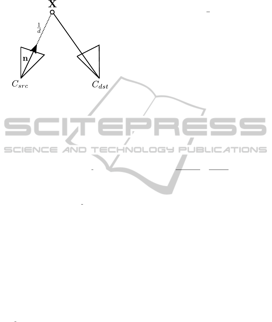
Figure 2: Inverse point parametrization with source camera
and destination camera.
but are generated as the same type of structure. Next,
different measurement types are described. We create
a measurement (quat:[cam],[0]) where the object
is a quaternion enforced to have unit length. The
indices written in the second pair of square brackets
specify the indices of the objects to be optimized.
The next measurement represents the error of the
reprojection in the image with fixed intrinsic parame-
ters (projMetric:[pt2,pt3,cam,cam in],[1,2]).
Only the objects pt3 and cam are part of the
optimization. Adjusting the measurement in a
way that the intrinsic parameters are optimized as
well, the last list is extended by the fourth object
(projRadial:[pt2,pt3,cam,cam in],[1,2,3]).
The user provides the system with information,
closely related to the bracket notation above. Using
OpenOF, it is easy and fast to test different kinds of
parametrizations.
We compare a new BA parametrization with the
one previously described. This new method is called
inverse bundle adjustment (IBA) due to the inverse
depth parametrization (Civera et al., 2008). A 3D
point is no longer described by three parameters, but
with a source camera, a unit vector and an inverse
depth. So the point is linked to the camera of first
appearance (see Fig. 2). For the parametrization we
end up with the following list:
• pt3inv:[d][nx,ny,nz]
• cam:[CX,CY,CZ,q1,q2,q3,q4]
• cam in:[fx,fy,u0,v0,s,k1,k2,k3]
• pt2:[x,y]
In this example we distinguish between fix and opti-
mizable parameters. For pt3inv, d is part of the opti-
mization, but nx,ny,nz remain constant. The coordi-
nates (X,Y, Z) of a 3D point are computed according
to
˜
X =
0
X
Y
Z
=
1
d
q
−1
˜
nq +
˜
C (14)
with q being the quaternion corresponding to the
source camera and C is the camera center. The tilde
above the variable denotes a quaternion representa-
tion of a 3D vector. The described parametrization
has several advantages. The degrees of freedom of the
complete optimization are reduced by 2n with n rep-
resenting the number of points. The part of the state
vector which holds the parameters of the cameras has
the same size, since a camera can be a source and a
destination camera at the same time. At the same time
the amount of measurements is reduced by n. The
measurement in the source camera is neglected. This
might be a disadvantage as more measurements make
the optimization more stable. Regarding the opti-
mization, more important is the ratio between param-
eters and measurements. Assuming that each point is
seen by each camera and n > 7, m > 3, with m be-
ing the number of cameras, the ratio of parameters to
measurements is always smaller for IBA than for BA.
7m + n
2n(m − 1)
<
7m + 3n
2nm
(15)
For Equation 15 we assumed that the intrinsic
camera parameters are fixed. We investigated a
depth parametrization as well but found the inverse
parametrization to be superior due to a more linear
behavior.
7 RESULTS
For evaluation we compare IBA to BA both computed
with OpenOF. Both methods are evaluated against
simulated data as well as a real world dataset. The
performance is compared against two open source BA
implementations, Simple Sparse Bundle Adjustment
(SSBA) (Zach, 2012) and PBA (Wu et al., 2011). The
latter stands for Parallel Bundle Adjustment imple-
mented for the GPU and CPU. In contrast to SSBA,
PBA uses CG as presented in our approach. We show
that the performance of the specially optimized PBA
is comparable to OpenOF. All evaluations are per-
formed on an Intel i7 with 3.07 GHz, 24 GB RAM
and an NVIDIA GTX 570 graphics card with 2.5
GB memory. For both versions of PBA as well as
for OpenOF we use single precision. In contrast
SSBA runs with double precision. For evaluation we
use synthetic data shown in Fig. 3. The 3D points
are randomly generated and placed on the walls of a
cube. The points are only projected into cameras for
VISAPP2013-InternationalConferenceonComputerVisionTheoryandApplications
264
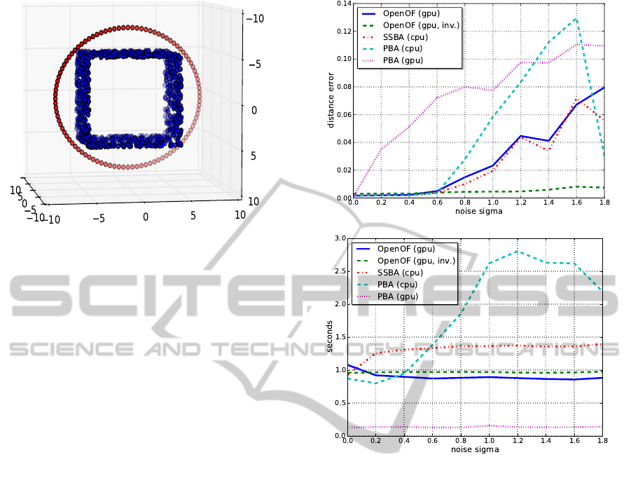
Figure 3: Setup of points (blue) and cams (red) for the sim-
ulated data.
which the points are directly visible in reality, assum-
ing the cube is not transparent. The cube has a size
of 10x10x10. The cameras are positioned on a cir-
cle with a radius of 8, facing the center of the cube.
The points are projected into a virtual camera with
an image size of 640x480 and a focal length of 1000
measured in pixels. The principle point is assumed to
lie in the center of the image. To simulate structure
from motion approaches, where the initial camera po-
sition is rather a rough estimate, we apply noise to the
camera position. Normally distributed noise of 0.5
pixels is applied to the measurement. Furthermore,
we triangulate new points from the virtual projections
instead of using the original 3D point, resulting in
a more realistic setup. With known positions of the
cameras, we investigate the convergence of the five
BA implementations stated earlier by continuously
increasing the noise of the camera position. Within
this simulation we use 100 cameras and 1000 points.
The overall estimate of each method is transformed
to the original cameras with a Helmert transforma-
tion. The mean distance error between the estimated
and true camera position is shown in Fig. 4(a) for
different amounts of noise. For each noise level the
mean of several iterations is plotted. Within our test
the GPU implementation of PBA did not converge in
most cases, which is shown in Fig. 4(a). The rea-
son for the failure could not be identified but we can
exclude a wrong usage as there is only a single line
of code which toggles PBA from a CPU version to
a GPU one. Every other method shows similar preci-
sion for σ < 0.6. For σ > 0.6, IBA shows a better con-
vergence than the other methods due to less degrees
of freedom. Especially the CPU version of PBA most
often did not converge for noise σ > 1.2. The con-
vergence problem of PBA causes also an increasing
time (Fig. 4(b)), while the other approaches stay con-
(a) Precision
(b) Performance
Figure 4: Applying normal distributed noise on the camera
positions (100 cameras).
stant in time. To evaluate the speed of the algorithms,
we run each method with a constant amount of noise
while concomitantly increasing the number of cam-
eras. This reduces the distance between two cameras
and increases the number of projections of one 3D
point. As expected, SSBA, using a direct solver im-
plemented on a CPU, shows the lowest performance.
Regarding this example, the CG approach (OpenOF
and PBA) operates much faster than a direct solver
(see Figs. 5(a) and 5(b)). The GPU version of PBA
cannot be taken into account because it did not con-
verge.
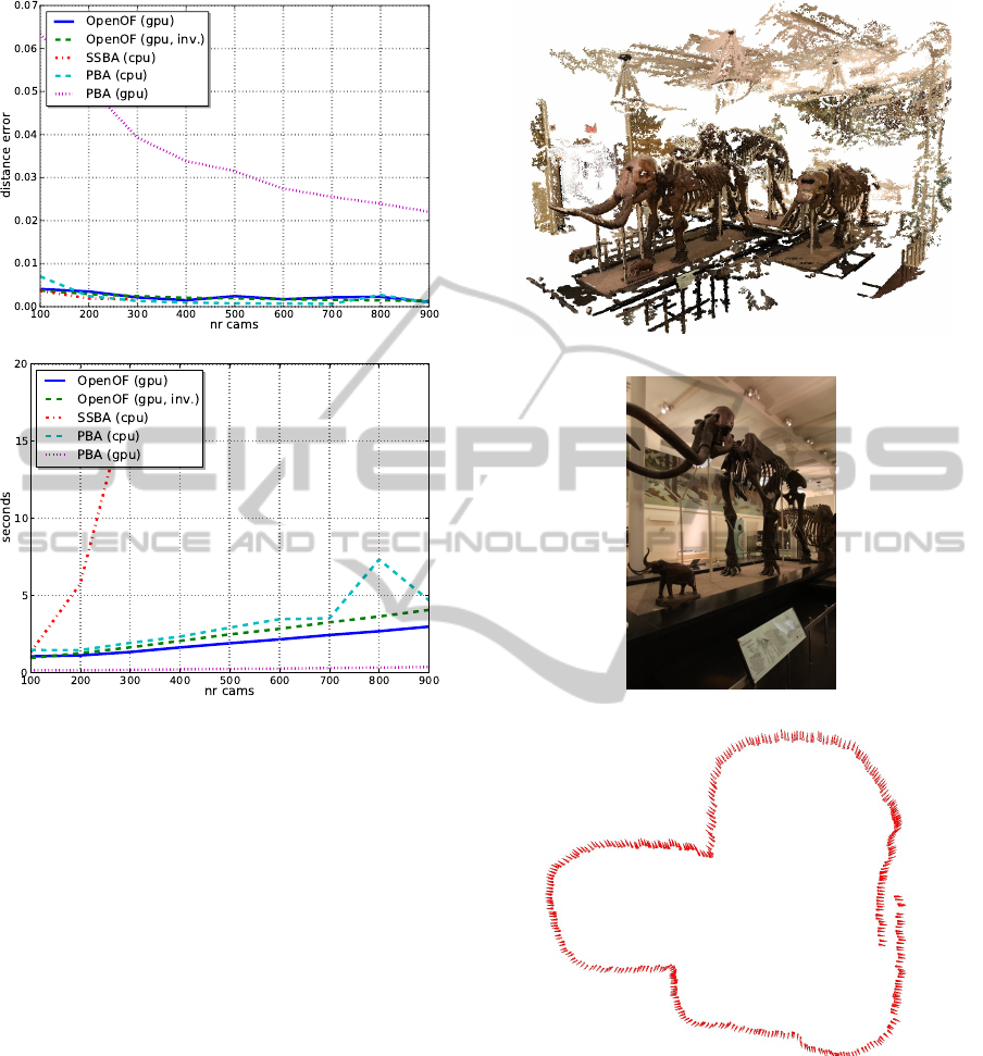
The real world data evaluation is performed on
a dataset with 390 images taken with a Canon EOS
7D camera (see Fig. 6(b)). The pictures were taken
in the American Museum of Natural History within
the scope of a project aiming at the reconstruction
of mammoths. Fig. 6(a) shows the final reconstruc-
tion computed with PMVS2 (Furukawa and Ponce,
2010). The path computed with OpenOF is illustrated
in Fig. 6(c). We compare the convergence rates be-
tween SSBA and OpenOF, respectively. PBA is not
OpenOF-FrameworkforSparseNon-linearLeastSquaresOptimizationonaGPU
265
(a) Precision
(b) Performance
Figure 5: Changing the number of cameras with constant
amount of noise on the camera position (σ = 0.5).
included in this part of the evaluation. It has an in-
ternally different error metric for the residuals so that
SSBA and PBA can not be compared at the same time.
As shown in Fig. 7(a), the convergence of SSBA and
OpenOF is similar for BA with respect to the num-
ber of iterations. Regarding the number of iterations
relative to the overall time, the CG approach outper-
forms the direct solver. This success is even larger for
datasets where the amount of overlapping images is
higher, as shown in the synthetic evaluation. The con-
vergence rate of IBA is better than of BA. This might
not hold in any case, but developers are encouraged to
try out different parametrizations to determine the op-
timal solution. Additionally a different parametriza-
tion for the rotation is feasible, e.g. Euler angles.
8 CONCLUSIONS
We present OpenOF, an open source framework for
sparse non-linear least squares optimization. The cost
functions to be optimized are described in a high
(a) Quasi-dense point cloud
(b) Sample image
(c) Camera path
Figure 6: Three mammoths acquired at the American Mu-
seum of Natural History.
level scripting language. Reducing the implementa-
tion time enables developers to comfortably try dif-
ferent modelings of functions. The estimates are
optimized on a GPU considering the sparse struc-
ture of the model. We showed that the generality
of OpenOF is not accomplished at the expense of
speed. OpenOF can compete with implementations
that are specifically designed for certain applications.
VISAPP2013-InternationalConferenceonComputerVisionTheoryandApplications
266
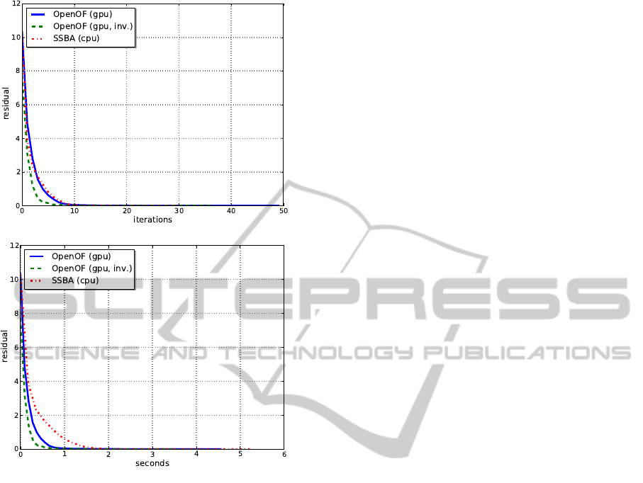
(a) Iterations
(b) Time
Figure 7: Convergence of the mammoth dataset.
OpenOF works successful on BA. A fair comparison
to the GPU version of PBA was not possible since
PBA did not provide reliable results. We will further
investigate why PBA shows just a poor convergence
behavior on our data. With IBA a new parametriza-
tion for BA has been introduced which often converge
for examples in which BA gets stuck in a local min-
imum. As in IBA the reprojection error of a point in
the source camera is zero, IBA probably does not find
the overall best solution. In practice we experienced
that IBA still converges for multiple datasets where
BA found a poor solution. In this case the result of
IBA can be further optimized with an additional BA
step.
The main aim of OpenOF is not to be another
BA implementation but to solve much more complex
least squares optimizations problems. Recently a fea-
ture has been added to OpenOF which allows the cost
function to include numerical parts. This is useful for
minimizing pixel differences in multiview stereo ap-
proaches. A set of various robust cost functions such
as Huber or a truncated L2 norm is available as well.
For future releases we want to integrate a CPU ver-
sion especially for developers which does not need
the speed, but want to have the flexibility in their de-
sign of cost functions.
REFERENCES
Civera, J., a.J. Davison, and Montiel, J. (2008). Inverse
Depth Parametrization for Monocular SLAM. IEEE
Transactions on Robotics, 24(5):932–945.
Davis, T. A. (2006). Direct Methods for Sparse Linear
Systems, volume 75 of Fundamentals of Algorithms.
SIAM.
Furukawa, Y. and Ponce, J. (2010). Accurate, dense, and ro-
bust multiview stereopsis. IEEE transactions on pat-
tern analysis and machine intelligence, 32(8):1362–
76.
Kaess, M., Johannsson, H., Roberts, R., Ila, V., Leonard, J.,
and Dellaert, F. (2011). iSAM2: Incremental smooth-
ing and mapping with fluid relinearization and incre-
mental variable reordering. In Robotics and Automa-
tion (ICRA), 2011 IEEE International Conference on,
pages 3281–3288. IEEE.
Kummerle, R., Grisetti, G., Strasdat, H., Konolige, K.,
and Burgard, W. (2011). g2o: A general framework
for graph optimization. In Robotics and Automa-
tion (ICRA), 2011 IEEE International Conference on,
pages 3607–3613. IEEE.
Lourakis, M. (2010). Sparse non-linear least squares op-
timization for geometric vision. Computer Vision -
ECCV 2010, pages 43–56.
Lourakis, M. I. A. and Argyros, A. A. (2009). SBA: A
software package for generic sparse bundle adjust-
ment. ACM Transactions on Mathematical Software,
36(1):1–30.
Madsen, K., Nielsen, H. B., and Tingleff, O. (2004). Meth-
ods for Non-Linear Least Squares Problems (2nd ed.).
Nocedal, J. and Wright, S. J. (1999). Numerical Optimiza-
tion, volume 43 of Springer Series in Operations Re-
search. Springer.
Wu, C., Agarwal, S., Curless, B., and Seitz, S. (2011). Mul-
ticore bundle adjustment. In Computer Vision and Pat-
tern Recognition (CVPR), 2011 IEEE Conference on,
number x, pages 3057–3064. IEEE.
Zach, C. (2012). Sources. http://www.inf.ethz.ch/personal/
chzach/ opensource.
OpenOF-FrameworkforSparseNon-linearLeastSquaresOptimizationonaGPU
267
