
Parametric Curve Reconstruction from Point Clouds using Minimization
Techniques
Oscar E. Ruiz
1
, C. Cort
´
es
1
, M. Aristiz
´
abal
1
, Diego A. Acosta
2
and Carlos A. Vanegas
3
1
Laboratorio de CAD/CAM/CAE, Universidad EAFIT, Carrera 49 No 7 Sur - 50, Medell
´
ın, Colombia
2
Grupo de Diseo de Productos y Procesos - DPP, Universidad EAFIT, Carrera 49 No 7 Sur - 50, Medell
´
ın, Colombia
3
City & Regional Planning, University of California, Berkeley, 228 Wurster Hall #1850, Berkeley, CA 94720-1850, U.S.A.
Keywords:
Parametric Curve Reconstruction, Noisy Point Cloud, Principal Component Analysis, Minimization.
Abstract:
Curve reconstruction from noisy point samples is central to surface reconstruction and therefore to reverse
engineering, medical imaging, etc. Although Piecewise Linear (PL) curve reconstruction plays an important
role, smooth (C
1
-, C
2
-,...) curves are needed for many applications. In reconstruction of parametric curves
from noisy point samples there remain unsolved issues such as (1) high computational expenses, (2) presence
of artifacts and outlier curls, (3) erratic behavior of self-intersecting curves, and (4) erratic excursions at
sharp corners. Some of these issues are related to non-Nyquist (i.e. sparse) samples. In response to these
shortcomings, this article reports the minimization-based fitting of parametric curves for noisy point clouds.
Our approach features: (a) Principal Component Analysis (PCA) pre-processing to obtain a topologically
correct approximation of the sampled curve. (b) Numerical, instead of algebraic, calculation of roots in point-
to-curve distances. (c) Penalties for curve excursions by using point cloud to - curve and curve to point cloud.
(d) Objective functions which are economic to minimize. The implemented algorithms successfully deal with
self - intersecting and / or non-Nyquist samples. Ongoing research includes self-tuning of the algorithms and
decimation of the point cloud and the control polygon.
GLOSSARY
PL : Piecewise Linear.
PCA : Principal Component Analysis
C
0
: Unknown planar curve to be fit.
S : {p
1
, p
2
,..., p
n
} noisy point sample of C
0
.
C(u) : Parametric planar curve approaching C
0
.
S
c
: {c
1
,c
2
,...,c
w
} PL disjoint curves
approaching local portions of C
0
.
L : PL curve, which integrates S
c
.
P : [q
1
,q
2
,...,q
m
] Control polygon of C(u).
µ : Stochastic component of S.
ε
k
: Error of minimization process at
iteration k.
B(p,r) : Disk of radius r centered at p.
Λ(λ) : p + λ. ˆv Parametric line starting at point
p, with direction ˆv and parameter λ.
pca(S
E
): PCA of point set S
E
. Returns p, ˆv and
correlation coefficient ρ.
r
i
: Residual associated to point p
i
∈ S
C
i
: Point on C(u) closest to cloud point p
i
.
d(p,S) : distance from point p to the point set S.
A
j
: set of points closest to p
j
.
1 INTRODUCTION
A considerable number of applications in CAD,
CAM, Medical Imaging and Geographic Information
Systems, deal with the sectioning of a non-self in-
tersecting shell (a 2-manifold ) in R
3
with cutting
planes. In Computer Axial Tomography (CAT), Co-
ordinate Measurement Machine (CMM) samples and
Magnetic Resonance Imaging (MRI), data sets (im-
ages, planar wire frames, cross cuts) planar curves
must be recovered from, i.e, noisy unordered point
samples.
Consider a planar curve C
0
sampled with a point
set S, which includes a stochastic noise with mean µ.
This article presents implemented algorithms to find
the b-spline curve C, a parametric approximation for
C
0
. The curve C is determined by its control polygon
P. The problem is tackled by tunning control points in
P to minimize f =
∑
n
i=1
r
2
i
where r
i
is obtained using
the distances between the cloud points p
i
∈ S and the
curve C. Besides considering for C
0
the usual open
smooth curves, this article addresses self-intersecting
and non-Nyquist ones. The method devised includes
35
E. Ruiz O., Cortés C., Aristizábal M., A. Acosta D. and A. Vanegas C..
Parametric Curve Reconstruction from Point Clouds using Minimization Techniques.
DOI: 10.5220/0004283900350048
In Proceedings of the International Conference on Computer Graphics Theory and Applications and International Conference on Information
Visualization Theory and Applications (GRAPP-2013), pages 35-48
ISBN: 978-989-8565-46-4
Copyright
c
2013 SCITEPRESS (Science and Technology Publications, Lda.)

saddle
point
M
p
s
(a) Saddle Point in 2-manifold M.
C
0
p
s
M
Π
(b) Cross Cut at Saddle Point.
S
(c) Self-intersecting Point Sample.
1st option: 1- manifold
non 1
- manifold
2nd option: 1- manifold
p
C
(d) Self-intersecting C and 1-manifold
Derivations.
Figure 1: Rationale for non-manifold curve reconstruction.
a pre-processing to find a topologically faithful initial
guess for P, a re-sample of P to minimize the number
of decision variables, a simplification of the calcula-
tion of distance p
i
to C and a calculation for r
i
that
includes distances to / from S to C.
1.1 Simple and Self-intersecting Curves
An open curve C : [a,b] ⊂ R → R
3
is simple if it does
not self - intersect, i.e., C(u
1
) = C(u
2
) ⇒ u
1
= u
2
for
all u
1
,u
2
∈ [a, b].
A typical scenario for self - intersecting curve re-
construction appears when a shell M (Fig. 1(a)), is
cross sectioned by planes. When a plane Π cuts the
shell M the result is a set of (open or closed) planar
curves. In general, those curves do not self - intersect.
However (Fig. 1(b)), if a horizontal plane Π passing
very near or at the saddle point p
s
cuts M, (nearly) self
- intersecting curves C
0
are produced. If the curves
are point-sampled, the sampling noise blurs their ex-
act geometry and topology. In such conditions it is
irrelevant whether or not the plane Π exactly contains
the saddle point p
s
: the point sample indicates a self -
intersecting curve (Fig. 1(c)).
Because of this reason, the recovery of self - in-
tersecting curves is relevant. The algorithms imple-
mented in this article are able to recover a self - in-
tersecting curve C -via its control polygon P- that re-
sembles C
0
(Fig 1(d), upper). The mutation of C into
1-manifold curve or curves is simple, as shown in the
lower curves in Fig 1(d).
1.2 Non-Nyquist Samples
A fundamental assumption in curve / surface recon-
struction from samples is that the Shannon / Nyquist
principle of digital sampling is respected ((Nyquist,
1928), (Shannon, 1949)). This principle establishes
that the spatial sampling interval δ
s
cannot be larger
than half of the smallest detail to be reconstructed.
The designer decides which is the size of the physi-
cal detail to reconstruct, and such a decision fixes the
δ
min =
0
δ
min =
0
δ
min
Figure 2: Examples of Nyquist / Non-Nyquist Shapes.
sampling interval δ
s
to use. Fig. 2 presents Nyquist
and non-Nyquist geometries. The left (croissant) one
has a very well defined non-null minimal detail dis-
tance δ
min
. Therefore, the sampling interval δ
s
can
comply with δ
s
< δ
min
/2 for a curve reconstruction to
be able to recognize the gorge region. The central fig-
ure (needle), on the contrary, presents δ
min
= 0. The
right figure (self - intersecting curve) also presents
δ
min
= 0. Therefore, for the center and right geome-
tries the sampling interval must be 0 = δ
s
< δ
min
/2,
and therefore we would require an infinitely tight
sample if the geometry and topology are to be fully
recovered. The self-intersecting curve (Fig. 2-right)
is obviously a non-manifold one. Notice that non-
manifoldness implies non-Nyquist. The contrary is
not true: a geometry may be manifold and yet non-
Nyquist (Fig. 2-center).
2 LITERATURE REVIEW
The problem of fitting a parametric curve C(u) to a
point cloud S has been addressed by many authors in
recent decades. However, as seen in this section, there
are many open issues in the solutions for such a prob-
lem.
2.1 Objective Function
Eq.1 is the general representation of the objective
function in curve fitting problems. Reference (Fl
¨
ory
and Hofer, 2010) employs first order residuals (w = 1)
while references (Wang et al., 2006; Liu et al., 2005;
GRAPP2013-InternationalConferenceonComputerGraphicsTheoryandApplications
36

G
´
alvez et al., 2007; Liu and Wang, 2008) use second
order residuals (w = 2).
f =
n
∑
i=1
r
w
i
(1)
Some references ((Wang et al., 2006; Liu et al.,
2005; Fl
¨
ory and Hofer, 2008; Fl
¨
ory and Hofer, 2010;
Fl
¨
ory, 2009)) add a smoothing term f
c
to the objective
function in order to adjust the roughness of the curve:
f =
n
∑
i=1
r
w
i
+ λ f
c
. (2)
The term f
c
contains information on the curve’s
first and/or second derivatives and λ determines its
influence, penalizing large curvatures. Notice that pe-
nalizing the curvature prevents curve fitting for non-
Nyquist samples.
Some authors have explored constrained ap-
proaches. Reference (Fl
¨
ory, 2009) presents con-
strained curve and surface fitting to a set of noisy
points in the presence of regions that the curve or sur-
face must avoid. Reference (Fl
¨
ory and Hofer, 2008)
considers the problem of curves that must lie on a
2-manifold (surface) with forbidden regions. These
procedures are implemented using a constrained non-
linear optimization strategy.
2.2 Distance Measurement
Eq.3 corresponds to the calculation of the distance d
i
,
which is usually used in the objective function in Eq.
1 as the residual r
i
. In curve fitting algorithms norm b
is usually chosen to be b = 2 (i.e., Euclidean distance)
as in (Wang et al., 2006; Liu et al., 2005).
d
i
= min
C(u)∈C
k
C(u) − S
i
k
b
(3)
However, the exact calculation of d
i
is expensive,
since it is obtained by a minimization procedure at
each fitting iteration. The procedure consists of find-
ing the parameter u
i
which associates a point on the
curve C(u
i
) with the i-th cloud point p
i
such that d
i
is
a minimum. Namely,
k
C(u
i
) − p
i
k
b
= min
C(u)∈C
k
C(u) − p
i
k
b
(4)
The minimum distance is obtained by performing
an orthogonal projection of the point p
i
to the curve
C, which occurs when C
0
(u
i
) · d
i
= 0 in Eq. 5.
g(u) =
C
0
(u) · (C(u) − p
i
)
(5)
To sort out this problem, one could solve for u in
g(u) = 0 using Newton’s Method ((Piegl and Tiller,
1997; Liu et al., 2005)), or minimize g(u) using nu-
meric methods ((Wang et al., 2006; Liu and Wang,
2008; Fl
¨
ory and Hofer, 2010; Saux and Daniel, 2003))
or using genetic algorithms ((G
´
alvez et al., 2007)).
The mentioned approaches have drawbacks inher-
ent to numerical methods, such as the need of a good
initial guess, poor convergence and stagnation at lo-
cal minima. These may lead to poor approximations
of the distance d
i
yielding unsatisfactory results of the
fitting procedure.
Different methodologies to measure the point-to-
curve distance have been proposed: (i) Point distance,
which preserves the Euclidean distance between the
cloud point and the paired point of the curve ((Wang
et al., 2006; Fl
¨
ory and Hofer, 2008)), (ii) Tangent
distance, which only preserves the distance between
the cloud point and the tangent line projected at the
paired point (Blake and Isard, 1998), and (iii) Squared
distance, which is a curvature-based quadratic ap-
proximation of d
2
i
((Wang et al., 2006)). Reference
(Liu and Wang, 2008) presents a comparison of these
methodologies.
It should be noticed that using only point-to-curve
distances to calculate f allows the formation of spuri-
ous curls and outliers (Fig. 8). Because of this reason,
we include also curve-to-point distances in f . This
double estimation allows us to avoid curls and out-
liers.
2.3 Initial Guess
In the present article the term initial guess refers to
a PL or smooth curve which approximates (possibly
with errors) the global point cloud. Numerical opti-
mization strategies require an initial guess to set the
decision variables. This set of values are chosen to
produce a reasonably good value of the function to
optimize, to then start the iterations. A good initial
initial guess has the capacity to offset the difficulties
posed by non-convex functions. If the initial guess
falls in a neighborhood in which the function is lo-
cally convex and a solution exists, the minimization
algorithms will be able to reach such solution, regard-
less of non-convexities of the function elsewhere.
In the particular domain of self - intersecting curve
fitting to noisy point clouds there are very few refer-
ences on how to find a reasonable initial guess for the
curve that is to be determined mathematical program-
ming.
References (Fl
¨
ory and Hofer, 2010; Wang et al.,
2006) start with a user - defined initial guess of the
curve sought. On the other hand, reference (Wang
et al., 2006) proposes to compute the quadtree parti-
tion of the point cloud and then extracts a sequence
ParametricCurveReconstructionfromPointCloudsusingMinimizationTechniques
37

of points which approximates the target shape. These
points are then used as initial control points of the fit-
ting curve. However, the autors do not report the im-
plementation of such method.
Ref. (Zhao et al., 2011) mentions the usage of
a 2D grid of uniform cells (i.e., not a quadtree), on
which the cloud points fall. The curve, therefore,
must lie on the set of cells which receive sampled
points. The centers of these cells are calculated and
interpolated to obtain the initial curve. However, the
strategy to order these center points is not presented.
It must be noted that the fitting of a PL or smooth
curve is precisely the problem of introducing a total
order among points which are representative of local
neighborhoods (either quadtree-based or cell-based)
of the point sample. The total order issue is partic-
ularly pressing for self-intersecting and non-Nyquist
curves.
2.4 Complexity Analysis
The complexity analysis allows to theoretically es-
timate the resources needed (time and memory) to
solve a problem using a given algorithm. It is cus-
tomary to express the performance of an algorithm
in terms of either (a) number of elementary opera-
tions, or (b) velocity of convergence. In case (a), an
operation is proposed as elementary for the solution
of the problem (e.g. comparison, assignment, query)
and then the number such operations required to solve
the problem for large problem sizes is computed in
the form of a function of n, the size of the problem
(O(n)). In case (b), a positive real number ζ is given,
meaning that the error in iteration k + 1 decreases
exponentially with respect to the error in iteration k
(ε
k+1
= (ε
k
)
ζ
), with 0.0 ≤ ε
k
< 1.0. Notice that using
(a) or (b) performance criteria avoids measuring the
execution time, which is influenced by the particular
hardware at hand. Instead, mathematical expressions
for (a) or (b), inherent to the problem, are used. De-
spite that, in general, the reviewed literature does not
address the topic of computational complexity of op-
timized parametric curve fitting, we will discuss some
considerations of several authors at this respect.
Liu et al. in (Liu and Wang, 2008) argue that the
computation of the Hessian using direct second order
derivatives of the parametric curve is a very expen-
sive operation. Because of this, they classify different
approaches to calculate the point-to-curve distance,
based on the usage or avoidance of the second deriva-
tives of C (see section 2.2). This reference does not
calculate the complexity of the different approaches
used. The other literature reviewed ((Park and Lee,
2007), (Fl
¨
ory, 2009), (Fl
¨
ory and Hofer, 2010), (Song
et al., 2009), (Liu et al., 2005), (Wang et al., 2006))
reports the execution times but does not conduct a for-
mal complexity discussion.
It is the case that pre-processings (e.g. initial
guess findings) are usually assessed in terms of O(n)
while minimizations are assessed in terms of ε
k
con-
vergence. In order to correctly estimate the com-
putational expenses for optimized curve fitting to
point clouds, we require the description of the com-
putational expenses for: (i) pre-processing (initial
guess generation) and (ii) optimization, on the same
grounds (either convergence speed of ε
k
or complex-
ity O(n)). Such an integration is not a trivial task.
2.5 Conclusions Literature Review and
Contribution of this Article
According to the taxonomy conducted in this litera-
ture review, there are several issues that remain open
in optimized curve fitting to point clouds. These as-
pects include: (a) Finding of topologically correct ini-
tial guesses to offset the fact that possibly f and / or
the minimization region are non - convex. (b) Usage
of a function f which efficiently fits the point set, al-
lowing for self - intersections and non-Nyquist sam-
ples. (c) Decimation of the number of control points
for C given that m control points imply a minimiza-
tion space of dimension R
2m
. (d) Formal assessment
of the computational time and space required for the
solution (e.g. O(n) analysis).
In response to the previous considerations, this
article reports the implementation of: (i) An initial
PCA-based initial guess for P and therefore C, which
is topologically faithful to the point set, being able to
follow self - intersections and non-Nyquist samples.
(ii) Decimation of excessive control points by the im-
plementation of a curvature-based re-sampling, to re-
duce the dimension of the search space. (iii) A dis-
crete calculation of the distance point-curve by using
a re-sampling of the curve. (iv) A double penalization
included in the objective function, based on the dis-
tances cloud-point-to-curve and curve-to-cloud-point,
therefore avoiding the existence of spurious curls and
outliers in C.
It must be pointed out that, although a significant
amount of work is required in the study of computa-
tional complexity, we do not intend to make a contri-
bution in such an aspect.
3 METHODOLOGY
The methodology used comprises the following
stages: (1) data pre-processing and (2) optimization
GRAPP2013-InternationalConferenceonComputerGraphicsTheoryandApplications
38

procedure. Stage (1) leads to a PL approximation of
the data to obtain a topologically correct initial guess
of the b-spline control polygon. Stage (2) implements
a Gauss-Newton optimization algorithm to minimize
the distance between the curve and the points S using
a penalized objective function. Fig. 3 summarizes the
procedure.
Preprocessing
Curvature-based
Resampling
PL Segments
Integration
PL Segments
Reconstruction
Gauss-Newton Algorithm
Jacobian
calculation
Objective Function
Evaluation
Stop criteria
met?
Curve noisy
point sample
Disconnected
PL Segments
Connected PL approximation
of the cloud points
Initial guess of
control polygon
Control Polygon
Update
New b-spline
approximation
No
Yes
Final b-spline
approximation
of the input data
Objective Function
Evaluation
Jacobian of
residuals
Figure 3: Block diagram of the proposed methodology.
3.1 Data Preprocessing
Given the S point set, an initial guess L for P (and
hence for C) is required, which is a rough PL approx-
imation of the curve C sought. This initial guess is
fundamental for the success of the optimization algo-
rithm that seeks C. L has correct topology, although
might not have a precise geometry. This initial guess
is calculated by a PCA pre-processing stage of our al-
gorithm.
Our approach is an extension of the work by (Ruiz
et al., 2011). The algorithm in (Ruiz et al., 2011) es-
timates the tangent to C at a particular point p of C
by running a PCA (i.e., generalized linear approxi-
mation Λ(λ) = p
cg
+ λ. ˆv with starting point at p
cg
,
direction ˆv and parameter λ) on the sample points of
such neighborhood. Those points are the subset of
S contained in a small circular ball B(r, p) based on
p. The goodness of the PCA can be evaluated using
a variation of the linear regression correlation coef-
ficient ρ. In a ’normal’ (i.e., 1-manifold conditions)
curve neighborhood, the linear approximation is very
good, and therefore ρ ≈ 1.0. In self - intersecting (i.e.,
non-manifold) or non-Nyquist curve neighborhoods,
the linearity falls and ρ ≈ 0. At such neighborhoods,
the support region choosing the points to participate
in the PCA mutates from circular into an elliptical
one. This is a key feature of the algorithm because
it permits to deal with self-intersections. The pro-
cess continues with the adjacent neighborhoods until
a dead end is found (i.e., no more points are available
in the current direction of search), and another region
is explored. The procedure is repeated until S is com-
pletely traversed, delivering a set of disconnected PL
curves, S
c
=
{
c
1
,c
2
...,c
h
}
, which approximates S.
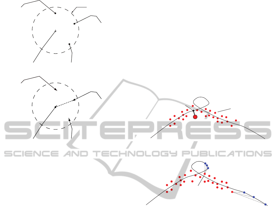
In the present article, we improve (Ruiz et al.,
2011) by adding a novel integration strategy for the
c
i
s to obtain a single connected approximation of C
0
,
defined as L. Let c
i
,c
j
,c
k
,c
l
be PL curve fragments
to be merged, which happen to have their endpoints
close to each other (see Fig. 4(a)). In this case, the
distance criterium is obviously insufficient to decide
which curve fragments should join. Therefore, an ad-
ditional criterium is used, namely the similarity of
tangent vectors at the curve endpoints. Based on it,
it is concluded that the pairs to join are (c
i
,c
k
) and
(c
j
,c
l
) for the example shown in Fig. 4(b). In the gen-
eral case, however, the c
i
curve fragments integrate
unambiguously.
The PL curve, L, integrating the c
i
s is topologi-
cally equivalent to C
0
, meaning that L has self inter-
sections if C
0
does. However, L is not a good approxi-
mation of C
0
in the geometrical sense (i.e., it does not
lie in the ’center’ of the point set S). Therefore, L by
itself does not solve the problem.
The initial guess of the control polygon P for C
is obtained by re-sampling L, since one wants to use
the bare minimum necessary control points that re-
tain the topology of C. The re-sample of L is con-
trolled by the curvature: low curvature (large curva-
ture radius) regions can be represented by fewer con-
trol points, and vice versa. Given a point p
i
of L, the
local radius of curvature, R
p
i
may be approximated
by the radius of the circumference defined by three
adjacent point samples, p
i−1
, p
i
, p
i+1
. The curvature,
K
p
i
is given by K
p
i
=
1
R
p
i
. The larger the K
p
i
, the
tighter of the re-sample of L. The initial and final
points of L are always included in the resulting re-
sampling. This curvature-based re-sampling strategy
ParametricCurveReconstructionfromPointCloudsusingMinimizationTechniques
39
c
j
c
i
c
k
c
l
R= δ
(a) Geometrically close endpoints.
û
i
û
j
û
k
û
l
(b) Similar end-tangents.
Figure 4: Criteria for integration of curve fragments c
i
.
strongly contributes to lower the computation time in
the subsequent optimized fitting since less variables
need to be estimated (see Fig. 5).
We name as P the re-sampled version of L. Also
to keep notation simple, we use P to note the different
instances of itself (P
1
, P
2
, .., P
k
, ...), formed as its ver-
tices are relocated during the optimization iterations
k. Notice also that P is the control polygon for curve
C.
3.2 Optimization Problem
The control polygon P resulting from the data pre-
processing in section 3.1 determines the topology of
C. The geometrical quality of P is, as expected, poor.
This means, the parametric curve controlled by poly-
gon P is not a principal curve for the point set S (i.e.,
does not cross the ’center’ of S). Therefore, the con-
trol points of P must now be used as decision vari-
ables to minimize the summation of the squared dis-
tances from the cloud points (i.e., points in S) to the
candidate curve C(u). A Gauss-Newton algorithm is
used to minimize the f function which expresses the
distances between the point cloud S and its approxi-
mating curve C.
The minimization problem is stated as follows:
GIVEN: A noisy point sample S = {p
1
, p
2
,..., p
n
} of
a planar parametric smooth (possibly self-intersecting
and with non-nyquist neighborhoods) curve C
0
.
GOAL: To determine the control polygon P that pro-
duces a b-spline curve C, minimizing
f =
n
∑
i=1
r
2
i
(6)
where r
i
is the residual or distance between cloud
point p
i
and the curve C. Informally, r
i
depends on
the distances from the cloud points in S to the curve
C and on the distances from the curve C to the point
clouds in C. As discussed later, these distances dif-
fer. Depending on the definition of r
i
, two different
strategies to minimize f arise, as discussed next.
parametric
curve
C
curl
outlier
leg
p
i
C(u
i
)
point
cloud S
(a) Distances Cloud Point to Curve.
outlier
leg
p
j
p
j
C(u
j
)
C(u
j
)
parametric
curve
C
(b) Distances Curve to Cloud Point.
Figure 6: Distances Cloud Points to/from Curve.
3.2.1 Strategy 1. Distance from Cloud Point to
Curve
We define the residuals as
r
i
= ||p
i
−C(u
i
)|| (7)
, where u
i
is the parameter in the domain of C which
defines the point C(u
i
) closest to p
i
. The term r
i
rep-
resents the distance measured from each cloud point
to the curve C (see Fig. 6(a)). This calculation of
the distance between a point and an algebraic curve is
a very expensive proposition because it implies the
calculation of common roots of a polynomial ideal
(see (Ruiz and Ferreira, 1996), (Kapur and Laksh-
man, 1992)). Notice that the vector p
i
−C(u
i
) is nor-
mal to the curve C at the point C(u
i
). To avoid the
computational expenses of algebraic root calculation,
we approximate C(u) in PL manner and calculate r
i
simply by an iterative process. We sample the do-
main for C(u), ([0,1]) getting U = [0,∆
u
,2∆
u
,...,1.0]
GRAPP2013-InternationalConferenceonComputerGraphicsTheoryandApplications
40
0 2 4 6 8 10
−2
−1
0
1
2
3
4
5
6
7
x
y
(a) Initial control polygon using L.
0 2 4 6 8 10
−2
−1
0
1
2
3
4
5
6
7
x
y
(b) Re-sampled version of L.
Figure 5: Curvature-based control point decimation to estimate the initial control polygon.
and approximate the current C curve with the poly-
line [C(0),C(∆
u
),C(2∆
u
),...,C(1.0)]. Calculating an
approximation of C(u
i
) for a given p
i
simply en-
tails to traverse [C(0),C(∆
u
),C(2∆
u
),...,C(1.0)] to
find the C(N∆
u
) closest to p
i
. This is an O(n) process
(n=number of points), less elegant but much cheaper
than solving an algebraic system of equations (O(e
e
n
),
n=number of polynomials, (Kapur and Lakshman,
1992)), and sufficiently accurate.
Fig. 6(a) displays the distance from a particular
(emphasized) cloud point p
i
to its closest point C(u
i
)
on the current curve C. Such a distance has influence
in f as per Equation 6. Notice, however, that p
i
and
C(u
i
) (and hence f ) do not change if large legs and
curls appear in the synthesized C. Therefore, con-
sidering only the distance from cloud points to the
curve in Equation 6 permits the incorrect formation
of outlier legs and curls. The following section cor-
rects such a shortcoming.
3.2.2 Strategy 2. Inclusion of Distance from
Curve to Cloud Point
This section discusses how to include in the r
i
resid-
uals the distances from the curve points C
i
to the
cloud points p
i
(see Fig. 6(b)) to penalize in f the
growth of spurious outlier legs and / or curls just de-
scribed. If one can make spurious legs and curls to
inflate the objective function f , the minimization of
f avoids them. For any point p ∈ R
n
, the distance of
this point to S is a well defined mathematical function:
d(p,S) = min
p
j
∈S
(||p − p
j
||). For the current discussion
the points p are of the type C(u
i
) (i.e., they are points
of curve C). The u
i
parameters to use are the sequence
U = [0, ∆
u
,2∆
u
,...,1.0], already mentioned.
Notice that d(p,S) = ||p
j
− p|| for some cloud
point p
j
∈ S. Let us define the point set A
j
(on the
curve C) as:
A
j
= {C(u) | u ∈ U ∧ d(C(u),S) = ||p
j
−C(u)||}
(8)
The set A
j
contains those points in the sequence
[C(0),C(∆
u
),C(2∆
u
),...,C(1.0)] that are closer to the
point p
j
∈ S than to any other point of S. We note with
Z
j
the cardinality of A
j
. Observe that some Z
j
might
be zero, since p
j
could be far away from be curve C
and no point on the curve would have p
j
as its closest
in S. The set of all A
j
s could also be understood as a
partition of the curve C.
With the previous discussion, a new definition of
the residuals r
i
, to be used in Eq. 6, is possible:
r
i
= ||p
i
−C(u
i
)|| + (
1
Z
i
) Σ
C
ω
∈A
i
||C
ω
− p
i
|| (9)
The ||p
i
− C(u
i
)|| in Eq. 9 considers the dis-
tance from cloud points in S to the curve C. The
term (
1
Z
i
) Σ
C
ω
∈A
i
||C
ω
− p
i
|| expresses distances from the
curve C to the cloud points in S. This term penalizes
the length of the curve, by increasing f .
p
2
p
1
C
1
C
2
C
3
C
4
C
5
C
6
C
7
C
8
C
9
C
10
C
11
C
12
C
14
C
13
p
7
p
6
p
5
p
4
p
3
C
16
C
15
Figure 7: Clusters of Distances form Curve to Cloud Points.
Fig. 7 presents a simplified materialization of the
situation. The previous discussion applied to Fig. 7
implies the calculations shown in Table 1. Observe
that C
i
= C(u
i
), the point on C closest to p
i
is not the
exact one but the approximation mentioned in previ-
ous paragraphs (using a tight PL approximation of C).
3.2.3 Jacobian in the Gauss-Newton Method
The Gauss Newton method uses the Hessian approx-
imation H ≈ J ∗ J
T
, which works well in the cases in
which the function or region Ω are not convex. Be-
cause in our case f is not convex, we choose this
ParametricCurveReconstructionfromPointCloudsusingMinimizationTechniques
41

Table 1: Calculations using curve to cloud-point distances for example in Fig. 7.
p
i
A
i
Z
i
C(u
i
) r
i
p
1
{C
1
,C
2
,C
3
,C
4
} 4 C
2
||p
1
−C
2
|| +
1
4
(||p
1
−C
1
|| + ||p
1
−C
2
||
+||p
1
−C
3
|| + ||p
1
−C
4
||)
p
2
{C
5
,C
6
,C
7
} 3 C
6
||p
2
−C
6
|| +
1
3
(||p
2
−C
5
|| + ||p
2
−C
6
||
+||p
2
−C
7
||)
p
3
{} 0 C
8
||p
3
−C
8
||
p
4
{C
8
,C
9
} 2 C
9
||p
4
−C
9
|| +
1
2
(||p
4
−C
8
|| + ||p
4
−C
9
||)
p
5
{C
10
,C
11
} 2 C
10
||p
5
−C
10
|| +
1
2
(||p
5
−C
10
|| + ||p
5
−C
11
||)
p
6
{C
12
,C
13
} 2 C
12
||p
6
−C
12
|| +
1
2
(||p
6
−C
12
|| + ||p
6
−C
13
||)
p
7
{C
14
,C
15
,C
16
} 3 C
14
||p
7
−C
14
|| +
1
3
(||p
7
−C
14
|| + ||p
7
−C
15
||
+||p
7
−C
16
||)
method for the minimization. The Gauss - Newton
method presents better convergence with small resid-
uals r
i
. Because of this reason, we use an good quality
initial guess (in this case, a PCA-based one), which
indeed produces low values in the residuals.
The Gauss-Newton optimization procedure em-
ploys an approximation to the Hessian matrix H. The
calculation of H implies several aspects: (i) it is ex-
pensive, (ii) it is actually a discrete approximation,
(iii) its usage in the search algorithm may mislead
it. Because of these reasons, for the present article
the Hessian matrix will be approximated as H ≈ J
T
J,
where J is the Jacobian of the residuals with respect to
the decision variables. This approximation produces a
faster convergence of the decision variables to a local
minima than using the exact Hessian. The variables
to tune f are the x and y coordinates of the control
points (q
i
= (x
i
,y
i
)) contained in the control polygon
P = [q
1
,q
2
,...,q
m
]. The Jacobian of residuals is cal-
culated as follows:
J =
∂r
1
∂x
1
∂r
1
∂y
1
∂r
1
∂x
2
∂r
1
∂y
2
···
∂r
1
∂x
m
∂r
1
∂y
m
∂r
2
∂x
1
∂r
2
∂y
1
··· ··· ··· ··· ···
··· ··· ··· ··· ··· ··· ···
∂r
n
∂x
1
∂r
n
∂y
1
∂r
n
∂x
2
∂r
n
∂y
2
···
∂r
n
∂x
m
∂r
n
∂y
m
(10)
The dimension of the J matrix is (n × 2m) where
n = number of cloud points and m = number of points
in the control polygon. The calculation of each com-
ponent of the Jacobian is made numerically, using the
approximation of the partial derivative
∂r
n
∂x
=
∆r
n
∆x
. No-
tice that the variation of all decision variables are the
same ∆x.
The transformation of the control polygon is made
using the Jacobian of the residuals with the expression
X
k+1
= X
k
−
J
T
J
−1
J
T
r (11)
The dimensions associated with Eq. 11 are: X
(2m × 1), r (n × 1). X = [x
1
,y
1
,x
2
,y
2
,...,x
m
,y
m
]
T
is
just a convenient form for writing P. Notice that r =
[r
1
,r
2
,...,r
n
]
T
.
3.2.4 Criteria for Algorithm Termination
The Gauss-Newton procedure will continue finding
new control polygons until either of the following
conditions is met: (a) the variation of the objective
function from iteration k to k + 1 falls under a thresh-
old (| f
k+1
− f
k
| ≤ f
L
), (b) the values of the decision
variable do not significantly change between iteration
k and k + 1 (|X
k
− X
k+1
| < δ
min
), (c) the iterations ex-
ecuted surpass a limit: (N
iter
> N
max
).
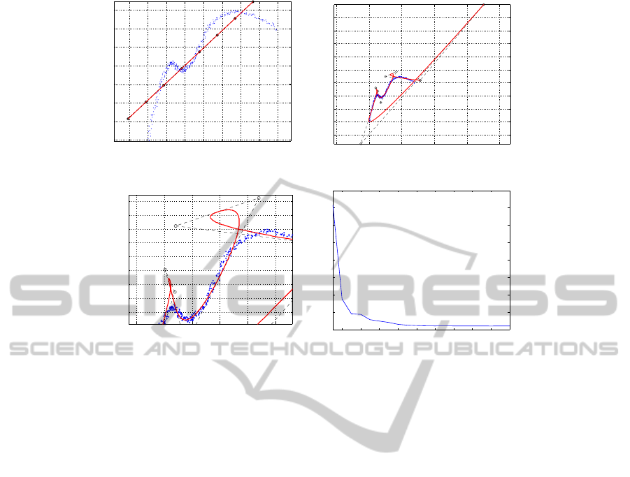
4 RESULTS AND DISCUSSION
4.1 Case Study 1. Simple Curves
4.1.1 Strategy 1. f based on Distance
Cloud-to-curve
The input data in this case of study corresponds to
a simple curve, as per Fig. 8(a). The initial (naive)
guess for the control polygon P is a straight segment.
It is obtained from an overall linear regression using
all cloud points. A sequence of points is sampled on
such a straight segment which constitutes the initial
control polygon P. The rationale for this initial guess
is that the optimization process will, progressively, re-
locate the control points, until the parametric curve C
resulting from P, approximating C
0
is achieved. The
mathematical problem solved has the form discussed
in section 3.2.1.
Notice that the case currently discussed uses the
simple form of the f function, in which only distances
from S to C are considered (excluding distances from
C to S), as per Eq. 7. The results, in Fig. 8(b), show
that the b-spline curve tends to follow the shape of the
cloud points at some regions, but its endpoints are lo-
cated far away from their correct positions and some
curls appear. As discussed before in section 3.2.1 and
GRAPP2013-InternationalConferenceonComputerGraphicsTheoryandApplications
42
−1 0 1 2 3 4 5 6 7
0
1
2
3
4
5
6
7
x
y
(a) Point Cloud and Naive Initial P guess.
−5 0 5 10 15 20
−2
0
2
4
6
8
10
12
14
16
x
y
(b) Synthesized C with curls and Outlier Legs.
0 1 2 3 4 5
4
4.5
5
5.5
6
6.5
7
7.5
8
x
y
(c) Close-up at curls of (b).
2 4 6 8 10 12 14 16 18 20
0
0.05
0.1
0.15
0.2
0.25
0.3
0.35
0.4
f
Iteration
(d) Objective Function f as function of iteration num-
ber.
Figure 8: Case Simple Curve C. Optimization uses naive initial guess and adds curve-to-cloud distance factor.
displayed in Fig. 6(a), such curls and otulier legs ap-
pear because the extent of C is not penalized in Eq.
7.
4.1.2 Strategy 2. f Suplemented with Distance
Curve-to-cloud
With point set S as per Fig. 9(a), the minimized curve
fitting is carried out now by adding curve-to-cloud
distances to the f objective function, as specified by
Eq. 9. This run uses the naive initial guess for P (i.e.,
sequence of colinear points). The resulting curve C is
correct, suppressing the curls and keeping the curve
attached to the ends of the input data. It is observed
that very few iterations are needed to yield satisfac-
tory results, showing fast convergence.
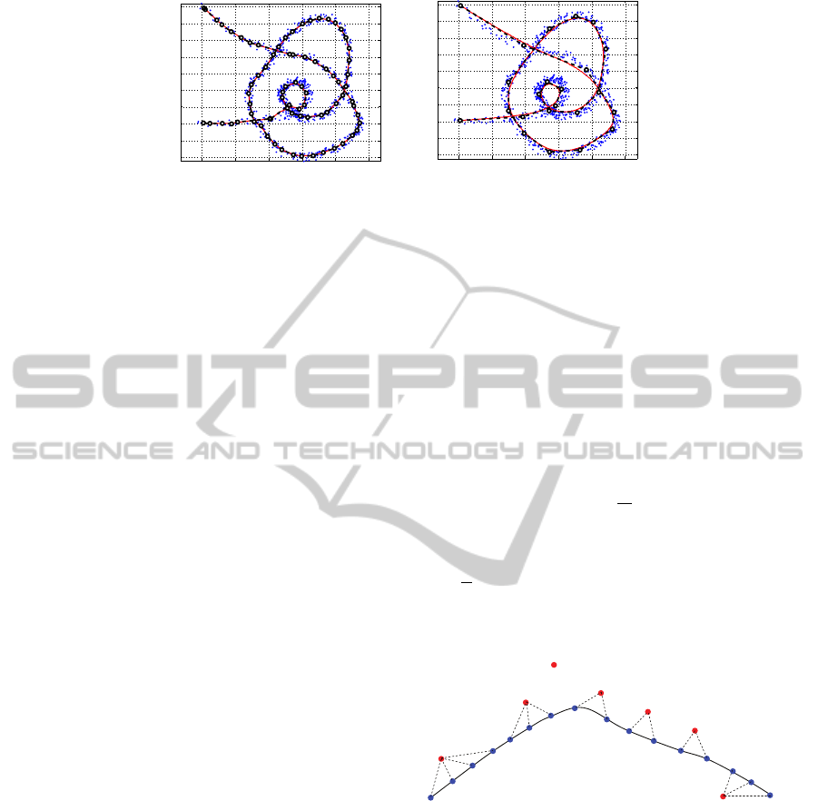
4.2 Case Study 2: Self-intersecting
Curve
The point set for this run series appears in Fig. 10(a).
As seen, it comes from a self - intersecting curve C.
The goal of this section is to evaluate the effects of a
smart initial guess for P, on the curve reconstruction
results. From now on, the form of the f function fo
minimize is the one in Eq. 9. This means, the dis-
tances cloud-to-curve and curve-to-cloud are used.
4.2.1 Naive Initial Guess for P
Fig. 10(a) shows the naive initial guess for the con-
trol polygon P (i.e., sequence of colinear points). No-
tice that a sufficient number of points must be sam-
pled on the segment. Too few sampled points ob-
viously prevent following the topological evolutions
of the curve. Too many control points considerably
degrade the performance of the minimization algo-
rithm, since this number of points equals the dimen-
sion of the solution space. Fig. 10(b) shows that with
this naive guess, the reconstruction of C
0
dramatically
fails, even if a sufficient number of control points are
provided on the straight segment of Fig. 10(a). Fig.
10(c) shows the evolution of f along the iterative pro-
cess.
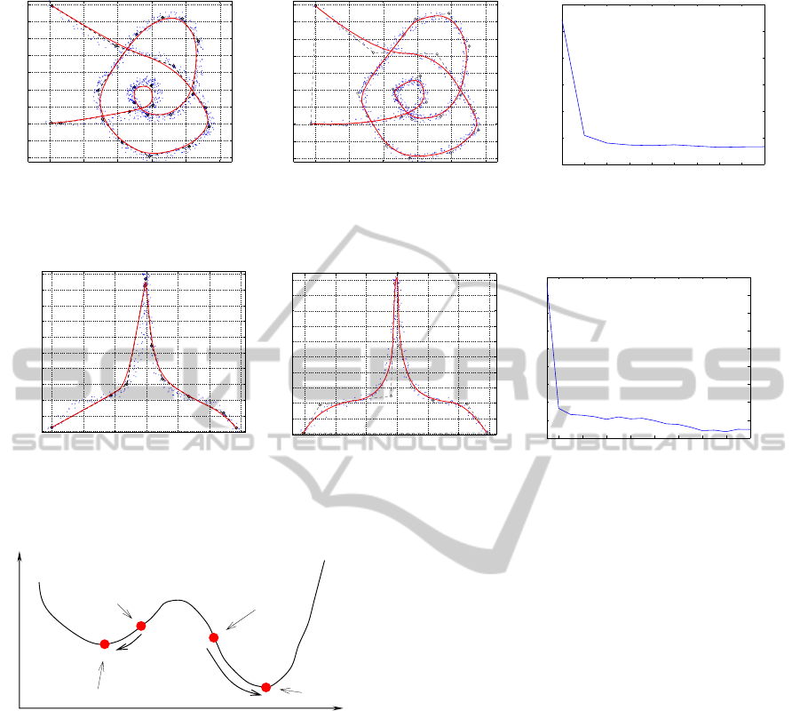
4.2.2 PCA-based Initial Guess for P
The goal of this run is to test the effect of having a
topologically correct initial guess for P, the control
polygon of C. Fig. 11(a) shows the point set sam-
pled on a self-intersecting C. This figure also shows
an initial guess for the control polygon P found by the
PCA-based pre-processing. Observe that this initial P
captures the correct topology, although not the right
geometry, of C. Therefore, one requires a minimiza-
tion stage to relocate the vertices of P. The resulting
ParametricCurveReconstructionfromPointCloudsusingMinimizationTechniques
43
−1 0 1 2 3 4 5 6 7
0
1
2
3
4
5
6
7
x
y
(a) Point Cloud and Naive Initial P guess.
−1 0 1 2 3 4 5 6 7 8
0
1
2
3
4
5
6
7
x
y
(b) Final control polygon P and its fit curve C.
2 4 6 8 10 12
0
0.05
0.1
0.15
0.2
0.25
0.3
0.35
0.4
0.45
f
Iteration
(c) Objective Function f as function of iteration num-
ber.
Figure 9: Case Simple Curve C. Optimization uses naive initial guess and adds curve-to-cloud distance factor.
−2 0 2 4 6 8 10
−2
−1
0
1
2
3
4
5
6
7
8
x
y
(a) Point Cloud and Naive Initial P guess.
−2 0 2 4 6 8 10
−3
−2
−1
0
1
2
3
4
5
6
7
x
y
(b) Final control polygon P and its fit curve C.
2 4 6 8 10 12
0
0.5
1
1.5
2
2.5
3
3.5
4
4.5
f
Iteration
(c) Objective Function f as function of iteration
number.
Figure 10: Open Curve with Self - intersection. C fit without PCA pre-processing.
control polygon P and its corresponding curve C ap-
pear in Fig. 11(b). Fig. 11(c) shows the history if f
as the iterations take place.
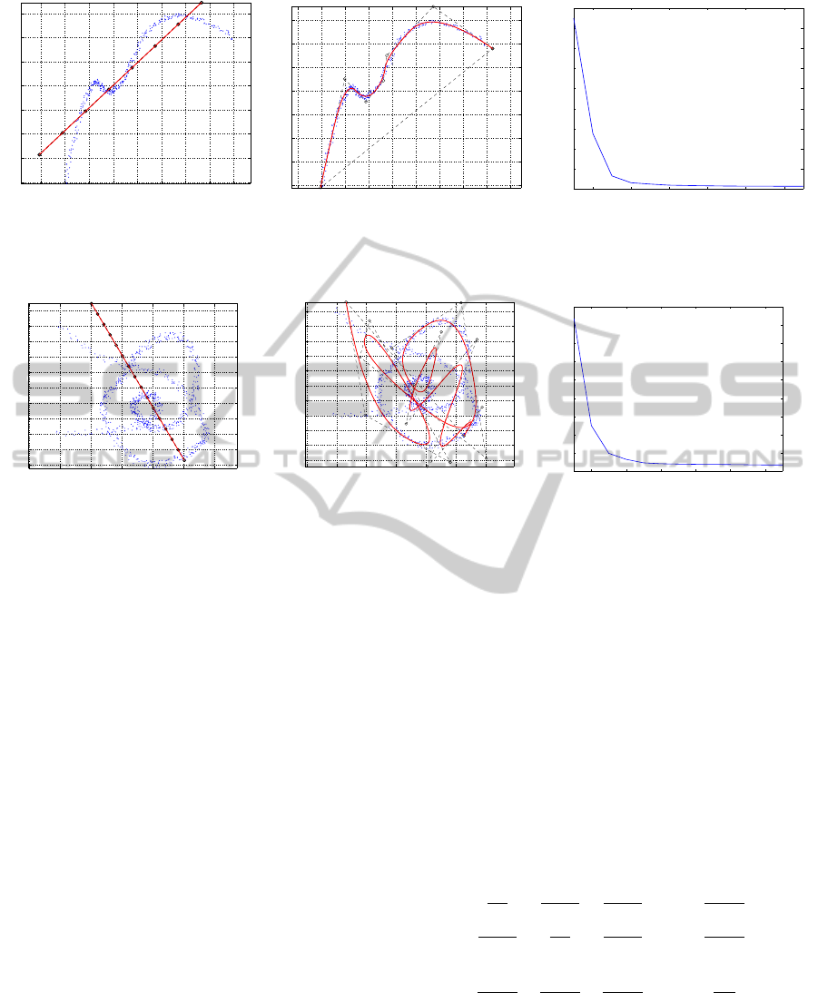
4.3 Case Study 3: Sharp-cornered
Curve
Fig. 12(a) presents a point sample for a curve that has
only C
0
continuity. The Nyquist principle ((Shannon,
1949),(Nyquist, 1928)) applied to geometry sampling
requires that at this point the sampling distance raises
to infinity and the sampling interval drops to zero,
implying that an infinitely tight sample would be re-
quired to recover all the geometric information of the
original curve C
0
. The obvious compromise indicates
that, since only a finite sample is available, part of
the needle is amputated in the curve-reconstruction.
Unfortunately, even accepting such an amputation, is
very likely that in such cases (of non-Nyquist sam-
ples), the topology of the curve cannot be recovered.
The present example represents a very difficult (non-
Nyquist) data set.
Fig. 12(a) presents the initial guess for the con-
trol polygon P originated using PCA. Fig. 12(b) dis-
plays the C the parametric curve finally achieved by
the minimization algorithm. Fig. 12(c) shows the his-
tory of the minimized f as function of the iteration.
As seen, since the application of PCA pre-processing
is able to correctly recover the topology of the curve
C, it is relatively straightforward for the minimization
process to tune up the vertices of P for the correct
placement of C. This efficiency is evident from the
fast convergence in very early iterations in Fig. 12(c).
4.4 Discussion
4.4.1 Initial Guess and Globality
The Hessian matrix for the problem in Eq. 6 is:
H =
∂
2
f
∂x
2
1
∂
2
f
∂x
1
∂y
1
∂
2
f
∂x
1
∂x
2
···
∂
2
f
∂x
1
∂y
m
∂
2
f
∂y
1
∂x
1
∂
2
f
∂y
2
1
∂
2
f
∂y
1
∂x
2
···
∂
2
f
∂y
1
∂y
m
··· ··· ··· ··· ·· ·
∂
2
f
∂y
m
∂x
1
∂
2
f
∂y
m
∂y
1
∂
2
f
∂y
m
∂x
2
···
∂
2
f
∂y
2
m
(12)
with the minimum search domain Ω being a subset
of R
2m
. If the eigenvalues of H are all positive in Ω,
one would be in presence of an overall convex func-
tion f and the minimization algorithm would rapidly
find the solution, guaranteed to be a global minimum.
Unfortunately, f as per Eq. 6 is not globally convex.
GRAPP2013-InternationalConferenceonComputerGraphicsTheoryandApplications
44
0 2 4 6 8 10
−2
−1
0
1
2
3
4
5
6
7
x
y
(a) Point cloud S and PCA-based initial control
polygon P
0 2 4 6 8 10
−2
−1
0
1
2
3
4
5
6
7
x
y
(b) Final control polygon P and its fit curve C.
1 2 3 4 5 6 7 8 9 10
0.02
0.03
0.04
0.05
0.06
0.07
0.08
f
Iteration
(c) Objective Function f as function of iteration
number.
Figure 11: Open Curve with self-Intersections. C fit using a PCA-based initial guess.
0 2 4 6 8 10 12
0
1
2
3
4
5
6
7
8
9
10
x
y
(a) Point cloud S and PCA-based initial control
polygon P.
0 2 4 6 8 10 12
0
1
2
3
4
5
6
7
8
9
10
x
y
(b) Final control polygon P and its fit curve C.
2 4 6 8 10 12 14 16 18
0.03
0.04
0.05
0.06
0.07
0.08
0.09
0.1
0.11
0.12
f
Iteration
(c) Objective Function f as function of iteration
number.
Figure 12: Non-Nyquist point set. C fit using a PCA-based initial guess.
local
minimum
global
minimum
PCA-based
initial
g
uess
naive initial
g
uess
P
f
Figure 13: Need of sensible guess with non-convex f .
Notice that H in Eq. 12 is not available and we use
H ≈ J
T
J instead. This replacement obviously does
not change the non-convexity of f .
Fig. 10 illustrates the effect of not having a glob-
ally convex function f . The initial guess for the poly-
gon P is not a sensible one, which means that the ini-
tial location in the Ω space is far from the minimum.
A poor initial guess for P produces a worng fitting
result, as shown in Fig. 10(b). This wrong result ex-
plains our need of the PCA-based pre-processing. Fig
10(c) shows that the solution is a local minimum. f
is indeed minimized in a wrong neighborhood, and
the solution for P (and C) is equally wrong. Fig. 13
shows that, precisely because the non-convexity of f ,
an intelligent initial guess for P is required for the
minimization algorithm to find a global minimum for
f . We claim here that the PCA-based pre-processing
improves the chances for an initial guess sufficiently
close to the global minimim and therefore partially
offsets the inherent difficulty represented by the non-
convexity of f .
4.4.2 Distance Curve to Point Cloud
As mentioned, the minimization using Eq. 7 per-
mits the formation of curls and leg outliers as per Fig.
8(b). This calculation of f includes only the distance
from the cloud points p
i
to the curve C. To prevent
these spurious formations we include in the f func-
tion the distance from the curve C to the point clouds
p
i
. The distance cloud-point-to-curve and curve-to-
cloud-point are not the same. Including the second
one (Eq. 9) makes f increase when outliers and curls
appear. This is a preventive rather than corrective
strategy, which ensures a correct topology and geom-
etry of the curve C.
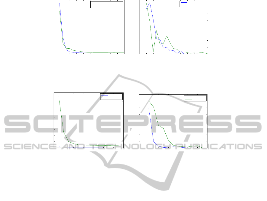
4.4.3 Comparative Convergence
Fig. 14 displays, for a simple curve, a comparison
between convergence speeds achieved using only dis-
tance cloud-point-to-curve (Eq. 7) versus including
also distances curve-to-point-cloud (Eq. 9). The
two cases are called without and with penalization,
ParametricCurveReconstructionfromPointCloudsusingMinimizationTechniques
45
0 2 4 6 8 10 12 14 16 18 20
0
0.05
0.1
0.15
0.2
0.25
0.3
0.35
0.4
0.45
Iteration
f
With penalization
Without penalization
(a) Double-distance Influence. Simple Curve.
0 2 4 6 8 10 12 14 16 18 20
0
0.1
0.2
0.3
0.4
0.5
0.6
0.7
0.8
Iteration
Relative delta f
With penalization
Without penalization
(b) Double-distance Influence. Simple Curve.
Convergence Speed.
Figure 14: Simple Curve Case. f as a function of iteration count. Influence of double-distance penalization.
0 2 4 6 8 10 12 14
0
0.5
1
1.5
2
2.5
3
3.5
4
4.5
Iteration
f
With PCA
Without PCA
(a) Initial Guess Influence. Self - intersecting
curve.
0 2 4 6 8 10 12 14
0
0.1
0.2
0.3
0.4
0.5
0.6
0.7
0.8
Iteration
Relative delta f
With PCA
Without PCA
(b) Initial Guess Influence. Self - intersecting
curve. Convergence speed.
Figure 15: Self - intersecting Curve case. f as a function of iteration count. Influence of PCA-based initial guess.
respectively. Fig. 14(a) shows that using the two
distances produces a faster reduction of the f fac-
tor. Fig. 14(b) indicates that the reduction in f
values more monotonous when penalization is used.
In other words, the optimization algorithm converges
faster to the solution. Notice that the convergence
when double-distance penalization is used (blue line),
the number of iterations required is 60% of the ones
required when only distance cloud-point-to-curve is
used (green line).
Fig. 15 illustrates, for a self - intersecting curve,
the comparison of convergence speeds by (1) using
PCA-based initial guess for the control polygon P and
by (2) abstaining from it. Fig. 15(a) indicates that, for
self - intersecting curves, the usage of a PCA-based
initial guess dramatically improves the convergence
speed of the optimization algorithm. Fig. 15(b) also
shows that the trend of the convergence is definitely
more monotonous when a PCA-based initial guess is
used. As in the discussion related to usage of double-
distance penalization of f , in this case (blue line) the
usage of PCA-based initial guess has an number of
iterations being 71% of the one required (green line)
when no sensible initial guess is used.
5 COMPLEXITY OF THE
ALGORITHM
Pre-processing. In Fig. 3, this stage refers to the
finding of an initial quess for P (and therefore C). A
sensible initial guess is found by (a) applying a PCA
algorithm to find PL fragments c
i
, (b) joining the dis-
connected c
i
fragments into one (L), and (c) re - sam-
pling the L to obtain a PL approximation for P. If we
assume that the number of cloud points is n, the com-
plexity of the ellipse-based PCA is O(n
4
) ((Ruiz et al.,
2011)). This complexity is dominant and therefore in-
cludes the integration of PCA-based curve fragments
and the curvature-based re-sample of the initial guess
for P.
Optimization. In Fig. 3, this stage refers to the
minimization of the f function by tunning the deci-
sion variables (i.e., control points of P) so that C fits
the point cloud S. This algorithm is controlled by a
while loop that stops when ε reaches a low value.
The calculation of the Jacobian, the update (which
implies a PL approximation) of the curve C and the
update of the function f together cost O(n
2
). There-
fore, the optimization stage costs O(g(ε) ∗ n
2
). Since
typically, g(ε) ∝ 1/(ε
2
), the complexity of the opti-
GRAPP2013-InternationalConferenceonComputerGraphicsTheoryandApplications
46

mization stage is O((n/ε)
2
).
According to the previous discussion, the over-
all complexity of the algorithm in Fig. 3 is O(n
4
+
(n/ε)
2
) = max(n
4
,(n/ε)
2
). Additional work is re-
quired to determine which one of n
4
and (n/ε)
2
is
dominant. A valid question to be posed is whether the
pre - processing might be removed, and its computa-
tional cost (O(n
4
)) spared. The answer is negative,
since a good quality initial guess for P is essential for
the optimization algorithm to converge to a topologi-
cally and geometrically valid solution. Fig. 10 illus-
trates the result for a run lacking a good quality initial
guess for P.
In the previous discussion, it must be pointed out
that the complexities considered are worst case ones.
Therefore, we present here a very conservative esti-
mation. For complexity estimation expected values
are also used.
6 CONCLUSIONS AND FUTURE
WORK
This article has presented the implementations of al-
gorithms to synthesize a parametric planar curve C as
an optimized fit for a point cloud S sampled from an
unknown initial curve C
0
. The curve C is therefore an
approximation for C
0
.
The implemented method presents several nov-
elties with respect to the existing contributions by
other authors: (1) It is successful in recovering
self-intersecting and non-Nyquist curves. (2) It
implements a Principal Component Analysis pre-
processing which finds a topologically faithful PL ap-
proximation for P, the control polygon of C. (3) This
initial guess for P is optimized in the sense of using a
very reduced number of vertices, which are chosen
according to the local curvature of P. (4) The al-
gorithm avoids the expensive calculation of distance-
point-curve, which implies algebraic roots, by calcu-
lating a PL approximation of curve C in each iteration
and solving the distance-point-curve with this proxy
approximation. (5) The algorithm penalizes f by con-
sidering not only the distances of cloud points p
i
∈ S
to C but also the distances from curve points C
i
to S.
Since C is finite, theses distances are not equal. By
doing so, the implemented method avoids the genera-
tion of spurious curls and outlier legs. Finally, (6) the
implemented algorithms lower the computation time
required to solve the problem by introducing features
(2), (3), (4), above.
Ongoing work includes exploration of other mini-
mization algorithms (Quasi-Newton for large values
of residuals), usage of different objective functions
to obtain faster convergence, improvement in self-
tunning of the algorithms, usage of unequal weights
in the residuals of Eq. 9 and a more aggressive strat-
egy to minimize the number m of the control points of
P. Since the search space is R
2m
, lowering m consid-
erably cuts the computing time for the minimization
of f .
REFERENCES
Blake, A. and Isard, M. (1998). Active contours: the ap-
plication of techniques from graphics, vision, control
theory and statistics to visual tracking of shapes in
motion. Springer.
Fl
¨
ory, S. (2009). Fitting curves and surfaces to point clouds
in the presence of obstacles. Computer Aided Geo-
metric Design, 26(2):192–202.
Fl
¨
ory, S. and Hofer, M. (2008). Constrained curve fitting on
manifolds. Computer-Aided Design, 40(1):25–34.
Fl
¨
ory, S. and Hofer, M. (2010). Surface fitting and registra-
tion of point clouds using approximations of the un-
signed distance function. Computer Aided Geometric
Design, 27(1):60–77.
G
´
alvez, A., Iglesias, A., Cobo, A., Puig-Pey, J., and Es-
pinola, J. (2007). B
´
ezier curve and surface fitting
of 3d point clouds through genetic algorithms, func-
tional networks and least-squares approximation. In
Proceedings of the 2007 international conference on
Computational science and Its applications-Volume
Part II, pages 680–693. Springer-Verlag.
Kapur, D. and Lakshman, Y. (1992). Elimination Methods:
An Introduction, pages 45–88. Academic Press.
Liu, Y. and Wang, W. (2008). A revisit to least squares
orthogonal distance fitting of parametric curves and
surfaces. In Chen and Juttler, editors, Advances in
Geometric Modeling and Processing, volume 4975 of
Lecture Notes in Computer Science, pages 384–397.
Springer Berlin / Heidelberg.
Liu, Y., Yang, H., and Wang, W. (2005). Reconstructing b-
spline curves from point clouds–a tangential flow ap-
proach using least squares minimization. In Proceed-
ings of the International Conference on Shape Mod-
eling and Applications 2005, pages 4–12. IEEE Com-
puter Society.
Nyquist, H. (1928). Certain topics in telegraph transmission
theory. Bell System Technical Journal.
Park, H. and Lee, J. (2007). B-spline curve fitting based
on adaptive curve refinement using dominant points.
Computer-Aided Design, 39(6):439–451.
Piegl, L. and Tiller, W. (1997). The NURBS book. Springer
Verlag.
Ruiz, O. E. and Ferreira, P. (1996). Algebraic Geometry
and Group Theory in Geometric Constraint Satisfac-
tion for Computer Aided Design and Assembly Plan-
ning. IIE Transactions. Focussed Issue on Design and
Manufacturing, 28(4):281–204. ISSN 0740-817X.
ParametricCurveReconstructionfromPointCloudsusingMinimizationTechniques
47

Ruiz, O. E., Vanegas, C. A., and Cadavid, C. (2011).
Ellipse-based principal component analysis for self-
intersecting curve reconstruction from noisy point
sets. The Visual Computer, 27(3):211–226.
Saux, E. and Daniel, M. (2003). An improved hoschek in-
trinsic parametrization. Computer Aided Geometric
Design, 20(8-9):513–521.
Shannon, C. (1949). Communication in presence of noise.
IRE, 37:10–21.
Song, X., Aigner, M., Chen, F., and J
¨
uttler, B. (2009).
Circular spline fitting using an evolution process.
Journal of computational and applied mathematics,
231(1):423–433.
Wang, W., Pottmann, H., and Liu, Y. (2006). Fitting
b-spline curves to point clouds by curvature-based
squared distance minimization. ACM Transactions on
Graphics (TOG), 25(2):214–238.
Zhao, X., Zhang, C., Yang, B., and Li, P. (2011). Adaptive
knot placement using a gmm-based continuous opti-
mization algorithm in b-spline curve approximation.
Computer-Aided Design.
GRAPP2013-InternationalConferenceonComputerGraphicsTheoryandApplications
48
