
Direct Estimation of the Backward Flow
Javier S
´
anchez, Agust
´
ın Salgado and Nelson Monz
´
on
Centro de Tecnolog
´
ıas de la Imagen (CTIM), Departamento de Inform
´
atica y Sistemas,
University of Las Palmas de Gran Canaria, Las Palmas de Gran Canaria, Spain
Keywords:
Backward Flow, Inverse Optical Flow, Back Registration, Inverse Mapping, Optical Flow, Image Registration,
Occlusions, Disocclusions.
Abstract:
The aim of this work is to propose a new method for estimating the backward flow directly from the optical
flow. We assume that the optical flow has already been computed and we need to estimate the inverse mapping.
This mapping is not bijective due to the presence of occlusions and disocclusions, therefore it is not possible to
estimate the inverse function in the whole domain. Values in these regions has to be guessed from the available
information. We propose an accurate algorithm to calculate the backward flow uniquely from the optical flow,
using a simple relation. Occlusions are filled by selecting the maximum motion and disocclusions are filled
with two different strategies: a min-fill strategy, which fills each disoccluded region with the minimum value
around the region; and a restricted min-fill approach that selects the minimum value in a close neighborhood.
In the experimental results, we show the accuracy of the method and compare the results using these two
strategies.
1 INTRODUCTION
In this article we address the problem of estimating
the backward flow. The optical flow is calculated
from the source to the target image and the back-
ward flow is the inverse mapping from the target to
the source image. If we know the forward flow, then
it is possible to estimate the backward correspondence
with some limitations.
This is important in problems where it is necessary
to find the correspondences back in time. This is the
case, for instance, in symmetric optical flow methods,
e.g. (Christensen and Johnson, 2001), (
´
Alvarez et al.,
2007b), (Ashburner, 2007) or (Yang et al., 2008).
These methods introduce the inverse optical flow to
improve the coherence between the forward and back-
ward flows.
In (Christensen and Johnson, 2001), for instance,
the authors present a method for computing the image
registration of medical images, which relies explicitly
in the computation of the inverse mapping. It works
for diffeomorphic transformations, where the relation
is bijective and differentiable. The backward flow is
calculated using an iterative algorithm, nevertheless,
this iterative process may slow down the method and
it does not work in occluded or disoccluded regions.
In the symmetric method presented in (Cachier
and Rey, 2000), the inverse optical flow is computed
using a Newton scheme. This solution is similar to
the previous iterative process, so it presents the same
drawbacks, providing poor results in occluded and
disoccluded regions. Another interesting symmetric
model is proposed in (
´
Alvarez et al., 2007a). In this
case, the optical flow is computed as a function in the
middle position between two frames, so it does not
compute the inverse optical flow explicitly.
The backward flow has also been used in spatio-
temporal optical flow methods, e.g. (Salgado and
S
´
anchez, 2006) or (S
´
anchez et al., 2013). The objec-
tive is to preserve the temporal coherence of the op-
tical flows with the previous estimated flows: the in-
verse optical flow is used to find the correspondences
back in time and impose some kind of temporal con-
tinuity.
Another example of the use of the backward flow
is given in (Lieb et al., 2005) and (Lookingbill et al.,
2007). In this case, the authors propose a method that
relies on the reverse optical flow to automatically fol-
low the road in autonomous cars. It tracks features
from the current position to a past position, so the
robot may identify similar shapes at different scales.
We propose a new method for estimating the back-
ward flow directly from the optical flow. We are given
the forward flow and we are interested in computing
268
Sánchez J., Salgado A. and Monzón N..
Direct Estimation of the Backward Flow.
DOI: 10.5220/0004284902680273
In Proceedings of the International Conference on Computer Vision Theory and Applications (VISAPP-2013), pages 268-273
ISBN: 978-989-8565-48-8
Copyright
c
2013 SCITEPRESS (Science and Technology Publications, Lda.)
the inverse optical flow with high precision. Nor-
mally, this is not an inverse function because there are
regions, like occlusions and disocclusions, where it is
not possible to establish a correspondence.
The proposed algorithm is simple, fast and ac-
curate. It automatically handles occlusions, whereas
disocclusions are filled using two distinct approaches:
on the one hand, we use a min-fill strategy, that asso-
ciates the minimum value around the region; on the
other hand, we propose a restricted min-fill approach,
that fills disocclusions with the minimum flow value
at a given distance.
In the experimental results, we study the pre-
cision of our method using synthetic standard se-
quences from the Middlebury benchmark database
(Baker et al., 2007). The results show that the accu-
racy of this method is high. We compare between the
solutions obtained by the two filling strategies. The
restricted min-fill approach provides better level of
accuracies when disoccluded regions are large.
In Section 2, we explain the basis for estimat-
ing the backward flow. The algorithm is designed in
Section 3 and the strategies to fill disocclusions are
explained in Section 4. In the experimental results,
Section 5, we evaluate the algorithm using several
sequences from the Middlebury benchmark datasets.
Finally, the conclusions in Section 6.
2 ESTIMATING THE BACKWARD
FLOW
The optical flow is the apparent motion of the objects
in a sequence of images. This is given by a vector
field, h(x) = (u(x),v(x)), that puts in correspondence
the pixels of a source and a target image. The back-
ward flow, h
∗
(x) = (u
∗
(x),v
∗
(x)), is the inverse map-
ping from the target to the source image. The relation
between the backward and forward optical flows is
given by
h(x) = −h
∗
(x + h(x)). (1)
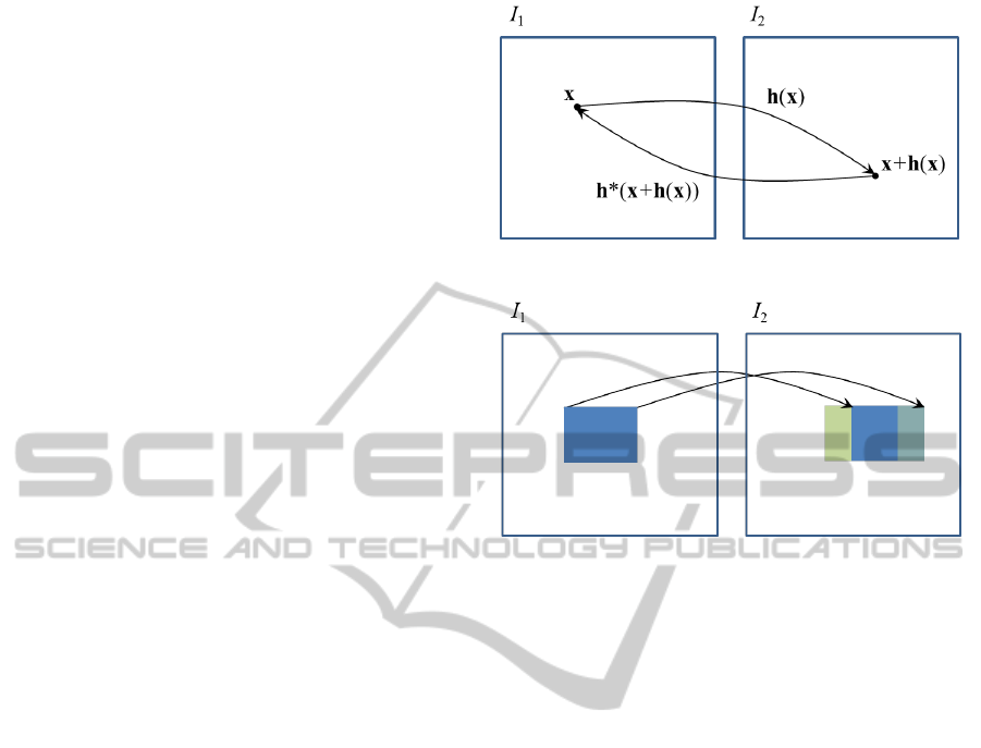
This relation can be intuitively derived from the
graphic depicted in Fig. 1: if we follow the path of
the forward and backward flows, we should arrive to
the initial position. This is true except in occluded
and disoccluded regions.
As depicted in Fig. 2, disocclusions appear in the
back side of the moving objects, produced by empty
regions where no correspondences can be established.
Occlusions appear in the front side of the moving
objects, where several correspondences arrive to the
same position. These two problems are easy to detect
Figure 1: Backward flow.
Figure 2: Occlusions and disocclusions. When the blue
square moves horizontally, it creates a disocclusion and oc-
clusion before and after the square, respectively.
but their solution have to be overcome from different
perspectives.
The disocclusion problem can be addressed as a
filling procedure, since the information is only avail-
able from the neighbors. Occlusions can be regarded
as a selection problem, where several values are as-
signed to the same position, and we need to select
the appropriate one. Occlusions occur because an ob-
ject moves in front of or behind other objects. In this
work we deal with occlusions due to objects moving
in front of other objects. This is a simpler case that
only depends on the vector field. The case, in where
an object moves behind other objects, is not so simple
and should rely on the image intensities as well.
3 ALGORITHM
Algorithm 1 shows the steps to compute the backward
flow. This algorithm is simple and very fast: only
one pass over the image is necessary to compute the
flow. The input is the forward flow. At the beginning,
we initialize the backward flow to a high number. In
each pixel, x = (x, y), we compute the corresponding
position in the other image, x + h(x).
We obtain the four neighbors around this position,
given by (x
+/−
,y
+/−
), and the interpolation weights,
w
1
,w
2
,w
3
,w
4
. These variables are shown in Fig. 3.
DirectEstimationoftheBackwardFlow
269
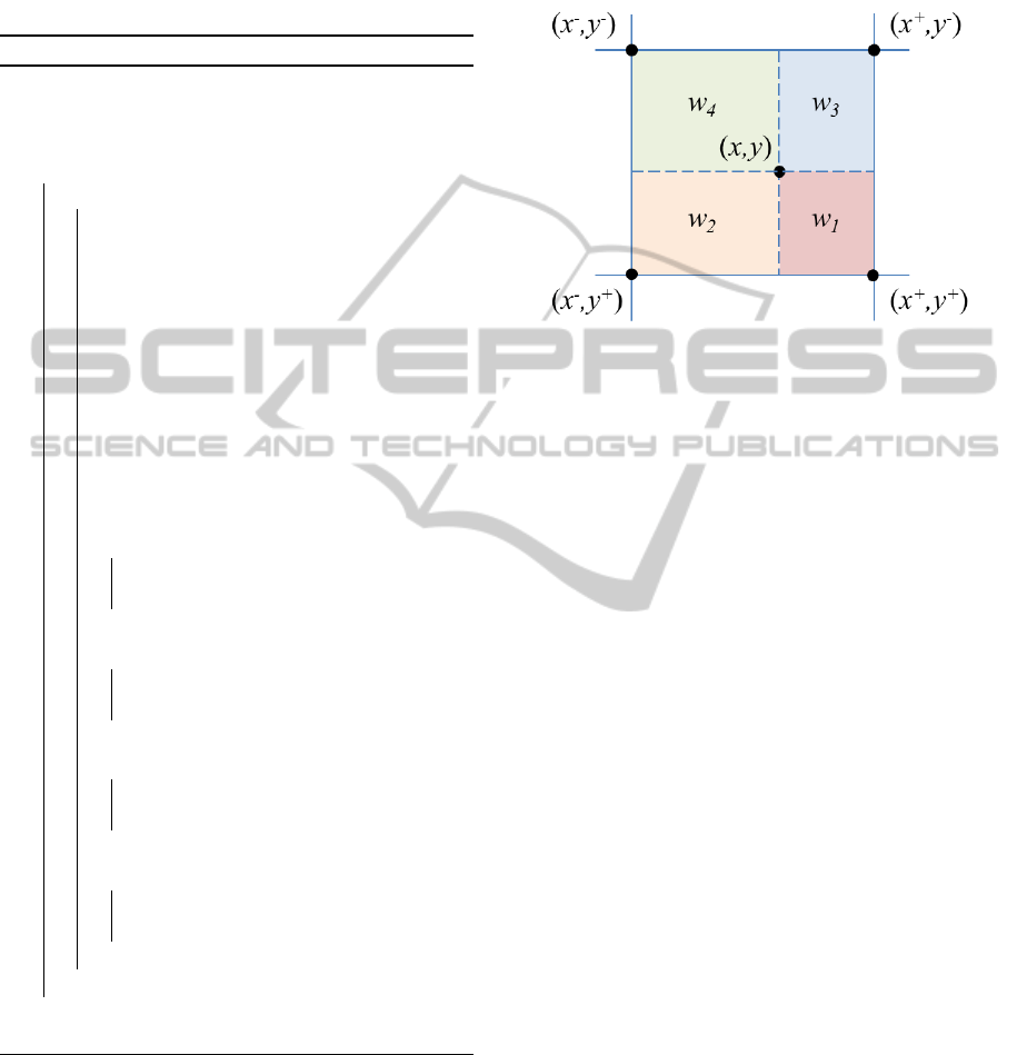
These weights represent the proportional area of the
pixel that corresponds to each neighbor. Then, we
estimate the magnitude of the forward flow and com-
pare it with the magnitude of the backward flows in
the neighborhood.
Algorithm 1: Backward flow estimation.
Input: u, v
Output: u
∗
,v
∗
Initialize u
∗
,v
∗
to a big number
for i ← 1 to size
y
do
for j ← 1 to size
x
do
x ← j + u( j, i)
y ← i + v( j,i)
Find the four neighbors of
(x,y) : (x
+/−
,y
+/−
)
Compute the bilinear interpolation
weights: w
1
,w
2
,w
3
,w
4
d ← u( j,i)
2
+ v( j,i)
2
d
1
← u
∗
(x
−
,y
−
)
2
+ v
∗
(x
−
,y
−
)
2
d
2
← u
∗
(x
+
,y
−
)
2
+ v
∗
(x
+
,y
−
)
2
d
3
← u
∗
(x
−
,y
+
)
2
+ v
∗
(x
−
,y
+
)
2
d
4
← u
∗
(x
+
,y
+
)
2
+ v
∗
(x
+
,y
+
)
2
if w
1
≥ 0,25 and d ≥ d
1
then
u
∗
(x
−
,y
−
) ← −u( j,i)
v
∗
(x
−
,y
−
) ← −v( j,i)
end
if w
2
≥ 0,25 and d ≥ d
2
then
u
∗
(x
+
,y
−
) ← −u( j,i)
v
∗
(x
+
,y
−
) ← −v( j,i)
end
if w
3
≥ 0,25 and d ≥ d
3
then
u
∗
(x
−
,y
+
) ← −u( j,i)
v
∗
(x
−
,y
+
) ← −v( j,i)
end
if w
4
≥ 0,25 and d ≥ d
4
then
u
∗
(x
+
,y
+
) ← −u( j,i)
v
∗
(x
+
,y
+
) ← −v( j,i)
end
end
end
Fill disocclusions
If the value of the forward magnitude is bigger
than the previous stored backward flow, and the corre-
sponding weight is bigger than a given threshold, then
we keep the negative value of the flow at that position.
This threshold has been set to 0,25 because it repre-
sents the situation where the correspondence falls in
the middle of the pixel.
In this way, the occlusions are automatically han-
dled by the algorithm: if there are collisions in one
position, we retain the flow with higher magnitude.
This is suitable when the occlusions are produced by
the fastest moving objects.
Figure 3: Notation.
Although this is not the most general case, it is in-
teresting because there are many sequences in which
this assumption holds. Also note that this algorithm
is very simple and fast, and the storage requirements
are very low, since all the information is stored in the
same output arrays. In the last step, the algorithm
fills disocclusions. These occur where no correspon-
dences have been found, thus it is the opposite situa-
tion to the occlusions.
4 FILLING DISOCCLUSIONS
In order to fill disocclusions, we have to look for the
values around the region. Normally, disocclusions
happen because a moving object let us see the back-
ground. The motion in this region cannot be dis-
covered, unless we make some simple assumptions.
The minimum flow assumption establishes that a good
guess is the minimum value around the disocclusion.
In this sense, we propose two strategies.
4.1 Min-fill Strategy
This strategy tries to fill disocclusions with the min-
imum value around the regions. This can be accom-
plished in the following steps: first, disocclusions are
grouped in regions by means of a connected compo-
nent labeling process (Suzuki et al., 2003).
The secod step consists in associating a minimum
value to each label: we go over the image and, any
time we find a disocclusion, we search for the mini-
mum value in its neigborhood and compare with the
accumulated minimum for its corresponding label.
VISAPP2013-InternationalConferenceonComputerVisionTheoryandApplications
270

Sequence Ground truth Backward flow Min-fill Restric. min-fill
Figure 4: Results for the Yosemite sequence. First column, the source image; second column, the ground truth; third column,
the computed backward flow without filling disocclusions (white color); fourth column, the backward flow with the min-fill
strategy; and, fifth column, the backward flow with the restricted min-fill strategy.
Once we have obtained the minimum value for
each label, we go over the image again and assign the
corresponding value to each disocclusion. This strat-
egy is simple and fast. It works correctly if the size of
the regions are small.
4.2 Restricted Min-fill Strategy
A simple strategy that works properly when regions
are very large, is the restricted min-fill strategy. The
idea is to find the minimum value that is near the cur-
rent position. For each disocclusion, we select the
minimum value in a window.
This process is carried out iteratively until every
disocclusion is filled: we go over the image and try
to fill disocclusions using a fix-sized window. The
size of the window may not be large enough to attain
values outside the region. In this case, the process
is run again to fill the remaining disocclusions. The
default window radius is 5 in the experimental results.
5 EXPERIMENTAL RESULTS
In the first experiment, Fig. 4, we use the Yosemite
sequence. Fig. 5 shows the color scheme used to
represent the orientation and magnitude of the vector
fields.
The average running times for the experiments is
about 0.020 seconds in a PC Intel Core i5 with two
processors and 8,00 GB RAM. These average times
include the time to read the input data and write the
output to disk.
Figure 5: Color scheme.
Table 1: EPE and AAE for the Yosemite sequence.
Min-fill Restr. min-fill
Sequence EPE AAE EPE AAE
Yosemite 0.084 0.529
o
0.012 0.307
o
Table 2: EPE and AAE for the Middlebury sequences.
Min-fill Restr. min-fill
Sequence EPE AAE EPE AAE
Grove2 0.035 0.560
o
0.026 0.417
o
Grove3 0.295 3.258
o
0.170 1.466
o
Urban2 0.294 1.547
o
0.086 0.345
o
Urban3 0.371 2.465
o
0.151 1.068
o
Venus 0.069 0.793
o
0.026 0.371
o
In order to evaluate the method, we compute the
backward flow twice, (h
∗
)
∗
, so that we arrive to
the original ground truth. Then, we compare with
the original ground truth using the average end-point
(EPE) and angular (AAE) errors (Baker et al., 2007),
for both strategies. Note that the estimated error mea-
sure may be divided by two to account for the actual
backward flow error. These results are shown in Ta-
ble 1. We observe that the restricted min-fill strategy
provides much better results than the min-fill strategy.
In Fig. 6, we show several results using the Mid-
dlebury benchmark database. We have used several
test sequences for which the ground truths are known.
In the third column of Fig. 6, we show the com-
puted backward flow with disocclusions highlighted
in white. The forth and fifth columns contain the solu-
tions for the min-fill and the restricted min-fill strate-
gies, repectively.
We observe that disoccluded regions are very large
in some examples. For instance, in the last sequence,
there is a large disocclusion in the border of the paper.
When this region is filled with the minimum value –
min-fill strategy – we observe a low motion (black
color), which is not consistent with the computed
backward flow around the region. The restricted min-
fill strategy seems to provide better results for this se-
quence.
In Table 2, we show the EPE and AAE for the
Middlebury sequences. We observe again that the re-
DirectEstimationoftheBackwardFlow
271
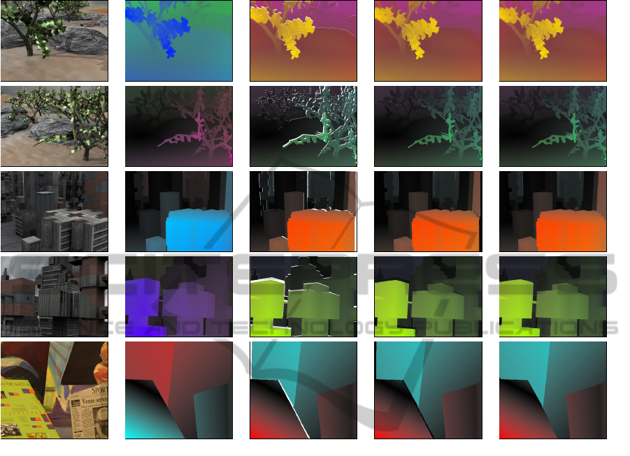
Sequence Ground truth Backward flow Min-fill Restric. min-fill
Figure 6: Results for the Middlebury test sequences. First column, the source image; second column, the ground truth optical
flow; third column, the computed backward flow without filling disocclusions; fourth column, the backward flow with the
min-fill strategy; and, fifth column, the backward flow with the restricted min-fill strategy.
stricted min-fill strategy attains better results than the
basic min-fill strategy.
6 CONCLUSIONS
In this work, we have presented a very accurate
method for estimating the backward flow. This
method only relies on the optical flow and can directly
deal with occlusions. On the other hand, in order to
fill dissoclusions, we have proposed two alternatives,
based on the minimum flow.
The algorithm is very fast, since it is only neces-
sary to carry out one pass over the image. This allows
us to reach real-time processing in current computers,
without the need to introduce any code parallelization.
In the experimental results, we have numerically
evaluated the new method and compared between the
two filling approaches. These results show that the
method is very accurate and that the restricted min-
fill approach provides better results.
The algorithm does not take into account occlu-
sions due to the movement of objects behind other
static objects. In this case, the information of the op-
tical flow is not sufficient and more information from
the images is necessary. This will be addressed in a
future work.
ACKNOWLEDGEMENTS
This work has been partly founded by the Spanish
Ministry of Science and Innovation through the re-
search project TIN2011-25488.
REFERENCES
´
Alvarez, L., Casta
˜
no, C. A., Krissian, K., Mazorra, L., Sal-
gado, A. J., and S
´
anchez, J. (2007a). Symmetric Op-
tical Flow. In Moreno D
´
ıaz, R., Pichler, F., and Que-
sada Arencibia, A., editors, Computer Aided Systems
VISAPP2013-InternationalConferenceonComputerVisionTheoryandApplications
272

Theory - EUROCAST 2007, volume 4739 of Lecture
Notes in Computer Science, pages 676–683. Springer
Verlag, Heidelberg.
´
Alvarez, L., Deriche, R., Papadopoulo, T., and S
´
anchez, J.
(2007b). Symmetrical dense optical flow estimation
with occlusions detection. International Journal of
Computer Vision, 75(3):371–385.
Ashburner, J. (2007). A fast diffeomorphic image registra-
tion algorithm. NeuroImage, 38(1):95–113.
Baker, S., Scharstein, D., Lewis, J. P., Roth, S., Black, M. J.,
and Szeliski, R. (2007). A database and evaluation
methodology for optical flow. In International Con-
ference on Computer Vision, pages 1–8.
Cachier, P. and Rey, D. (2000). Symmetrization of the non-
rigid registration problem using inversion-invariant
energies: Application to multiple sclerosis. In Delp,
S., DiGoia, A., and Jaramaz, B., editors, Medical Im-
age Computing and Computer-Assisted Intervention
MICCAI 2000, volume 1935 of Lecture Notes in Com-
puter Science, pages 472–481. Springer Berlin Hei-
delberg.
Christensen, G. and Johnson, H. (2001). Consistent image
registration. IEEE Transactions on Medical Imaging,
20(7):568 –582.
Lieb, D., Lookingbill, A., and Thrun, S. (2005). Adaptive
road following using self-supervised learning and re-
verse optical flow. In Proceedings of Robotics: Sci-
ence and Systems, Cambridge, USA.
Lookingbill, A., Rogers, J., Lieb, D., Curry, J., and Thrun,
S. (2007). Reverse optical flow for self-supervised
adaptive autonomous robot navigation. International
Journal of Computer Vision, 74:287–302.
Salgado, A. and S
´
anchez, J. (2006). A temporal regularizer
for large optical flow estimation. In IEEE Interna-
tional Conference on Image Processing ICIP, pages
1233–1236.
S
´
anchez, J., Salgado, A., and Monz
´
on, N. (2013). Op-
tical flow estimation with consistent spatio-temporal
coherence models. In 8th International Conference on
Computer Vision Theory and Applications (VISAPP).
Suzuki, K., Horiba, I., and Sugie, N. (2003). Linear-time
connected-component labeling based on sequential lo-
cal operations. Computer Vision and Image Under-
standing, 89(1):1–23.
Yang, D., Li, H., Low, D. A., Deasy, J. O., and Naqa,
I. E. (2008). A fast inverse consistent deformable im-
age registration method based on symmetric optical
flow computation. Physics in Medicine and Biology,
53(21):6143.
DirectEstimationoftheBackwardFlow
273
