Faustmann Optimal Pine Stands Stochastic Rotation Problem
Eduardo Navarrete and Jaime Bustos
Department of System Engineering, FRONTERA University, Francisco Salazar 01145, Temuco, Chile
Keywords: Optimal Tree Cutting, Logistical Diffusion, Real Options.
Abstract: The Faustmann optimal rotation harvesting pine stands models under Logistic and Gompertz wood stock
and Brown price stochastic diffusion processes are reformulated as stochastic one dimensional optimal
stopping problem, which are solvable with the Hamilton-Jacobi-Bellman equations. The stochastic models
predict a significant increase of the deterministic optimal cut, with 47.0% and 48.0% in the cases of the
Logistical and Gompertz wood stock diffusion respectively. The application of these models to a Chilean
forest company shows discrepancies due to the absence of consideration to wood stock and price
uncertainties that the company actual cut policy shows. The experimental data significantly validate the
Faustmann stochastic logistic model. They give a better approximation of the company cut policy,
underestimating it by 8.09% and producing a more reliable saturation volume than the Gompertz model.
The sensitivity analysis shows that both volatilities have a similar linear effect in the optimal cut, but the
wood stock volatility volume elasticity of 0.687 almost doubles the stumpage price volume elasticity of
0.350, showing the importance of this uncertainty.
1 INTRODUCTION TO RADIATA
PINE STANDS EXPLOITATION
The need to incorporate uncertainty in wood stock
and price is not new. Samuelson (1976) not only
validated Faustmann’s deterministic formula (1995)
as the correct one, but also considered that the
forestry economist’s “simple notion of stationary
equilibrium needs to be replaced by the notion of
perpetual Brownian motion”. The majority of the
early papers considered only price stochastic
diffusion and simple harvest rotation see (Clark and
Reed, 1989); Others like (Morck & Schwartz,1989);
(Insley, 2002; and Alvarez et al., 2006) considered
also wood stochastic diffusion. Few of them (Insley
& Rollins, 2005; Willasen, 1998) formulated these
problems as stochastic impulsive control and
considered price and wood stock stochastic diffusion
for the multiple rotation or Faustmann model. In a
previous paper Navarrete (2011) extended the single
and multiple optimal rotations harvesting pine stands
models without the stands’ regeneration cost for
Logistic wood stock and Brown price stochastic
diffusion processes, and reformulated it as an
optimal stopping problems with only one stochastic
diffusion, solvable with the Hamilton-Jacobi-
Bellman differential equations.
The objective of this paper is to extend those
stochastic results to the Faustmann formula with the
stands regeneration cost for Logistic and Gompertz
wood stock and Brown price diffusions, to solve the
stochastic rotation of even aged pine stands
harvesting and to validate these results by applying
them to a Chilean forest company.
2 METHODOLOGY
2.1 Model Formulation
Given the following variable and parameters
Vt = Wood stock at time t
µ(Vt) = Wood stock diffusion drift parameter
σ(Vt) = Wood stock volatility parameter
Pt = Wood stumpage spot price at time t
Po = Initial stumpage wood price
α = Wood price diffusion drift rate
β = Wood price volatility
W = Wiener diffusion
C = Stands regeneration cost
c = C/Po
R, Q = Probabilistic metrics
F = Functional Objective
57
Navarrete E. and Bustos J..
Faustmann Optimal Pine Stands Stochastic Rotation Problem.
DOI: 10.5220/0004285402050212
In Proceedings of the 2nd International Conference on Operations Research and Enterprise Systems (ICORES-2013), pages 205-212
ISBN: 978-989-8565-40-2
Copyright
c
 2013 SCITEPRESS (Science and Technology Publications, Lda.)

The model considers ITO diffusion for the wood
stock and a geometric Brown diffusion for the wood
price respectively, given by equations (1) and (2).
dV
t
= µ(V
t
)dt + σ(V
t
) dW (1)
dP
t
= αP
t
dt + βP
t
dW (2)
Under the assumption of a weak solution (Vt, t) for
the diffusion equations (1, 2) and initial conditions
(V0

0, P0

0), the multiple actualized harvest
value or Faustmann model (3), (see Johnson, 2006)
is given by objective functional (3).
00
sup ( )
(,) ( )
() 1
Rrt
F
tt
rt
o
EePV C
FVP
tt e




 
(3)
2.2 Reformulation of the Multiple
Harvest Rotation Problem
The stochastic model (1, 2, and 3) is difficult to
solve. The following theorem reduces this model
to a one dimensional stopping problem that is more
amenable.
Theorem 1: A probabilistic measure Q exists and
is equivalent to the actual metric R, such that: (see,
Appendix A)
)
1
(sup[
)
1
(
)(
sup
),(
)(
0
00
rt
t
tr
Q
rt
tt
rt
R
o
e
Ve
EP
e
VPe
E
tt
PVF









(4)
Furthermore, under the metric Q, the process V
t
follows the diffusion (5).
WdVdtVVdV
tttt
)()}()({  
(5)
An optimization strategy previously developed by
the author (see Navarrete, 2011) was used. The
functional objective (3) was parameterized for
different time values t=t
n,
generating a family of n
stochastic optimization problems. Since
)1/(
n
rt
eC


is constant for each t
n,
we can apply
theorem 1 and reformulate each of these problems as
the following optimal stopping problem with one
dimensional ITO diffusion.
F
F
(V) = sup (E
P
[
n
rt
e

P
t
V
t
]-C)/(1-
n
rt
e

))
= P
o
sup{E
Q
[
n
tr
e
)(  
V
t
/(1-
n
rt
e

)]– C/(1-
n
rt
e

}
(6)
Dividing by the constant Po, this objective is
reformulated as
F(V) = Max { E
Q
[
n
tr
e
)(  
V
t
/(1-
n
rt
e

)]
– c/(1-
n
rt
e

)}
(7)
with the following wood stock diffusion under the
metric Q.
WdVdtVVdV
tttt
)()}()({  
(8)
The formulation of the Hamilton Jacobi Bellman
equation for this problem is given by the following
inequation with the capitalized interest rate r
t
= r/ (1-
n
rt
e

).
Max{ ½σ
2
V
2
F´´(V) + [µ(V) + βσ(V)] F´(V)
– [r
t
-α] F(V) – c r
t
, (V-c)/(1-
n
rt
e

)-F(V)} = 0
(9)
In this case the differential equation for the
continuation region (V< V*) is given by the non
homogenous differential equation (10).
½σ
2
V
2
F´´(v) + [µ(V)+βσ(V)] F´(V)
- (r
t
-α) F(V) – c r
t
= 0
(10)
with F(0) = -(r
t
/r)c.
And by equation (11) for the stopping zone (V< V*).
(V-c)/ (1-
n
rt
e

)-F (V) = 0
(11)
The solution of this ordinary differential equation
under the initial condition for a given capitalized
interest r
t
is given in (12), with ψ(V) the solution of
the homogenous part and [ r
t
/r]c the particular
solution of equation (10).
F
F
(V,r
t
) = {
*)1/()(
*]/[)(
VVecV
VVcrrVA
rt
t





(12)
In this case the smooth pasting condition for each
parameter r
t
is given by:
AΨ (V*)-(r
t
/r) c = (V*-c)/ (1-e
-rt
) = (r
t
/r) (V*-c) and
Aψ´ (V*) = r
t
/r . So V*
t
must fulfill a similar
smooth-pasting condition to the Vicksell model for
each parameter r
t
.
Ψ (V*) = V* ψ´ (V*) (13)
This solution series is then optimized for the
Faustmann functional objective equation (7) under
metric Q by inspection of its values.
ICORES2013-InternationalConferenceonOperationsResearchandEnterpriseSystems
58

Figure 3.1: VOLUME (m3/ha) versus years, single plot.
3 EXPERIMENTAL DATA
AND PARAMETERS FITTING
3.1 Logistic Diffusion Fitting
The experimental data was provided by a Chilean
forest company. These data belongs to 128 harvest
stock of its pine stocks stands between 1999 and
2005 and came from different sample plots which
belong to site indexes between 30 and 35 meters and
represent sites with high forest aptitude and a tree
average initial volume of 32 m3/ha after the end of
the first 4 years initial seed cultivation period. This
information is located outside the 95% range of
confidence for the logistic adjusted figure, forming
an initial series of 122 data points, which are plotted
in figure 3.1.
dV = µ V (1- γ V) dt + σ Vdw (14)
The basic requirement of a pine stand growing
diffusion is its sigmoid pattern (Garcia, 2005). The
logistic diffusion, equation (14) is a special case of
the sigmoid model given by µ(V) = µV(1-γV) and
σ(V) = σ V, where µ and γ are the drift and
saturation parameters and σ is the volatility
parameter.




t
t
t
m
dsWsExpV
WtExpV
V
])
2
[([1
)
2
[(
2
0
2
0






(15)
The integration of the value of V is given by
equation (15) (Kloeden& Platen, 1991, page 125)
and its expected value is given by equation (16)
)(
1
1
)(
m
tt
t
e
VE





(16)
With; 1/γ = saturation volume, µ = growth rate
parameter = L
n
(81)/Δ
t
, Δ
t
= time necessary to
increase volume from 10% to 90% of saturated
volume and t
m
= time to achieve the midpoint of the
saturation volume.
The standard deviation Sd(∞) at the saturation
zone is constant and σ can be easily estimated by
equation (17).
σ = Sd(∞)/V
s
= (95% saturation confidence
interval)/(2 *1.96 *Vs)
(17)
The logistic diffusion model was fitted using a
logistical nonlinear regression and a Monte
Carlo/Bootstrap simulation sampling method,
implemented by Meyer et al. (Loglet Lab.1 software,
1999).
The result is presented in figure 3.2, showing the
drift parameter and its 95% confidence interval for
the whole series and for its saturation zone. The
summary of the parameter fitting is shown in table
3.1.
200
250
300
350
400
450
500
550
600
650
700
19 20 21 22 23 24 25 26
A
GE (years)
VOLUME (m3/ha))
FaustmannOptimalPineStandsStochasticRotationProblem
59

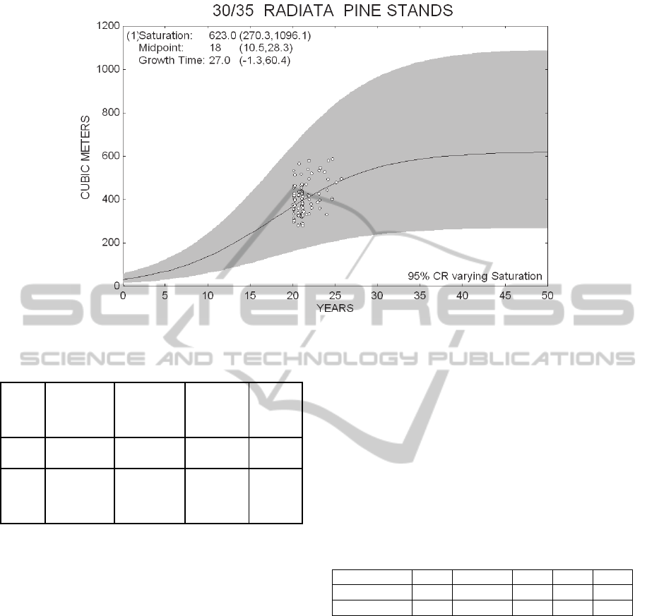
Figure 3.2: Expected logistic fitting for the stands 30/35 site.
Table 3.1: Logistic fitting parameters.
Site
Index
mts.
Drift
Parameter
µ
Drift
Saturation
Parameter γ
Saturation
Standard
Deviation
Volatilit
y
σ
30/35
0.163 0.00161 210.66 0.339
Deter
minist
ic
0.163 0.00161 0.00 0.00
See Navarrete 2011
3.2 Gompertz Diffusion Fitting
Another important sigmoid diffusion is the
Gompertz geometrical diffusion, which is given by
the following equation (18)
dV=kV[θ-ln(V)]dt + σVdW (18)
This equation is integrated to the following
expression, (see Gutierrez 2009)
V(t)= exp[ ln(V
0
)e
-
k
t
+ {(kθ-σ
2
/2)/k} (1-e
-k
t
)
+ σe
-kt
∫dW]
(19)
The expected value takes the following expression
E[V(t)]= exp [ln(V
0
)e
-kt
+ {(θ-σ
2
/(2k)}(1-e
-
kt
) + (σ
2
/(4k))(1-e
-2kt
)]
(20)
Taking natural logarithm and rearranging it, we get
ln E[V(t)]= A- Bx-Cx
2
(21)
with A= θ-σ
2
/(4k), B=θ-σ
2
/(2k) - ln(V
0
), C=σ
2
/(4k)
and x= e
-kt
Given a value for k, a quadratic fitting for e
-kt
and
e
-2kt
can be done estimating the value of A, B and C
until a common value for θ can be obtained from A
and B, determining the estimation for θ, k and σ.
The deterministic parameter only requires a linear
fitting with e
-kt,
. Both fittings were done for the
initial value V
0
= 32 (m3/ha.) and the results are
summarized in table 3.2.
Table 3.2: Gompertz Diffusions Parameters Estimations.
M
odels V
0
V
s
k θ σ
Gompertz 32.00 1046.68 0.058 7.0 0.171
D
eterministic 32.00 1083.09 0.058 6.984 0.000
3.3 Gompertz versus Logistical
Diffusion Fitting
The expected drift growing pattern of the Logistic
and Gompertz Wood Stock diffusion are shown in
figure 3.3.
Both models have fitting advantages and
disadvantages.
The Logistic model is a better representation of
the sigmoid growth pattern of the tree stands and
produces a more reliable estimation of the saturation
zone. Unfortunately they cannot be adjusted by
maximum likelihood estimates, and must be adjusted
by a Bootstrap simulating sampling method, see
(Beskos et al., 2006), similar as the one used.
ICORES2013-InternationalConferenceonOperationsResearchandEnterpriseSystems
60

Figure 3.3: Wood Stock growing diffusion pattern.
The Gompertz model can be fitted by common
statically features, such as Maximum likelihood. See
Gutierrez, et al, (2008) or a Quadratic fitting, which
were the methods used. It also presents a better
adjustment to the experimental data given its lower
volatility parameter, but it produces a worst
estimation equal to 1046.6 m3/ha of the saturation
zone for the tree growth stands, which was not
validated by the experimental data used. Given its
higher initial estimation of the growth parameter and
its lower volatility parameter it will always produce
a lower stochastic optimal solution than the Logistic
model.
3.4 Wood Price Diffusion Fitting
The stumpage stands price Brown diffusion
parameters were estimated by Navarrete, (2011).
The summary of Brown diffusion parameters for the
pulp commercial and stumpage prices is given in
Table 3.3 and for actual stumpage price in table 3.4.
Table 3.3: Stumpage Price Diffusion Parameters.
Summary
Stumpage
logs
Saw logs
Pulp
logs
Percentage 100 % 83.9 16.1
Price drift α 2.9% 3.08 1.79
Volatility β 15.9% 16.52 12.74
See Navarrete 2011
Table 3.4: Stumpage Actual Price Estimation.
YEARS
Saw log
price
(83.9%)
US$/m3
Pulp log
price
(16.1%)
US$/m3
Stumpage
log price
(100%)
US$/m3
2007 43 20 39.30
2008 46 22 42.14
2009 41 21 37.78
Average 39.74
Source: IFOP Anuario Forestal 2010
The regeneration costs of Radiata Pine Stands in
2009 are given in table 3.5
Table 3.5: Radiata Pine Stands Regeneration Cost.
Stands regeneration cost C US$/ha 882
Actual stumpage log price
P
T
US$/ha 39.74
Initial stumpage price P
0
US$/ha 21.43
c=C/P
0
41.16
Source: CEFOR-UACH
3.5 Capital Cost Estimation
The capital cost is estimated by using the CAPM
model for the Chilean Forest industrial sector. The
risky rate of return “r” was estimated as the
international Weight Average Cost of Capital
WACC given the high volatility of actual financial
markets.
Chilean equity capital cost K
e
= R
f
+ β( E(R
m
) –
R
f
)= 3.3+(1.01) 6 = 9.4
0
200
400
600
800
1000
1200
1400
0 20 40 60 80 100
WOOD VOLUME (m3/ha)
AGE (years)
GOMPERTZ
LOGISTIC
LOGISTIC
FaustmannOptimalPineStandsStochasticRotationProblem
61

Chilean Company WACC= 0.76 (12.4)
+0.24(7.6) (1-0.17) = 11%
International Company WACC = r = 11.8 ~12%
Source: CMPC Corp Search June 2009
4 STOCHASTIC RADIATA PINE
HARVESTING RESULTS
4.1 Wood Stock Logistic and Brown
Price Diffusion
Two of the more common sigmoid diffusion
processes used in this area (see Garcia, 2005) are the
Gompertz and the Logistic geometric diffusion. The
logistic geometric diffusion wood stock diffusion
parameters are; µ(V) = µV (1- γV) and σ
V
= σ V.
The Faustmann deterministic optimum is given
by the optimization of the deterministic functional
objective in equation (22).
t
rt
tt
tt
r
e
r
CVP
VP





)1(
)´(
(22)
Replacing it in the equation (22) P
t
= P
o
e
αt
and V
t
´ =
µV
t
(1-γV
t
) we finally obtain
V
t
= {(α+µ-r
t
) + √[(α+µ-r
t
)
2
+ 4µγcr
t
e
-αt
]}
/(2µγ)
(23)
In the stochastic case, the positive function ψ (V), is
the solution of the homogenous component (24) of
the differential equation (10), (see Navarrete 2011)
½ σ
2
V
2
F´´(v) + [µV(1-γV) + β σV] F´(V) -
(r
t
-α) F (V) = 0
(24)
The solution of equation (24) is given by the
Kummer expression (25)
ψ(V) = V
θ
KummerM {
2
2


V
, θ, 2θ
+
2
)(2





}
(25)
with θ the positive root is given by equation (26)
2
2
22
)(2
)
2
1
(
2
1













r
(26)
The Faustmann deterministic optimum is obtained
by intersecting curve (24) with the logistic curve
(16). The solution is programmed in Maple 15 for
both curves, and the optimum obtained is V* =
245.7 m
3
/h. The Faustmann stochastic solution, in
(13), for different values of the capitalized interest r
t
= r/ (1-e
-rt
) is programmed in Maple 15, using its
KummerM function. The optimum is obtained by
evaluating the Faustmann functional objective under
the Q metric (20) for the different V*
t
solutions of
equation (13). The summary of all optimal cuts
results for the aggregate 30/35 site index series of
the multiple rotation harvest or Faustmann formula
is given in table 4.1.
These results show that the Faustmann
deterministic optimum underestimates the actual
policy cut by 37.47% and its stochastic optimum
also underestimates the actual average cut by 8.09%,
so that the Stochastic optimum is 47.0 % bigger than
the deterministic value.
Table 4.1: Multiple Harvest Rotation Optimal Results
Wood stock Logistic diffusion.
Optimum
Stands
cuts
m
3
/ha
Percentage
Increase
%
Percentage
Increase %
Deterministic 245.7 -37.47 100
Actual 392.9 100
Stochastic 361.12 -8.09 47.0
4.2 Wood Stock Gompertz and Brown
Price Diffusion
In this case the parameters of the diffusion are: µ(V)
= k V (θ- ln(V)), and σ(V) = σ V. The deterministic
optimum is obtained by replacing P
t
=P
0
e
αt
andV =
exp (ln(V
0
)e
-kT
+ θ(1-e
-kT
) in equation (22) resulting
equation (28). Which intersection with equation (20)
gives the optimal volume V
opt
.
V ={r
t
ce
-αt
+ k(θ - ln(V
0
)) exp(θ – kT - (θ -
ln(V
0
))e
-kT
}/{r
t
- α}
(27)
The stochastic increasing function ψ(V), in this case,
is given by the solution of the homogenous part of
the differential equation (10) or equation (28).
½ σ
2
V
2
F´´(v) + [kV(θ - ln(V)) + β σV]
F´(V) - (r
t
- α) F (V) = 0
(28)
Choosing θ´= θ - σ
2
/(2k) + βσ/k and r = r
t
- α, the
equation is similar to the exponential Ornstein
Ulhembeck equation whose positive solution ψ(V)
is given by equation (29), (see Johnson, 2005)



eVzbaKummerM
eVzbaKummerUbba
V



),,(
),,()}1(/)1({
{)(
(29)
with a= (r
t
- α)/(2k) b= 0.5 and z= (k/σ
2
) [θ -
σ
2
/(2k)+ βσ/k-ln(V)]
2
.
ICORES2013-InternationalConferenceonOperationsResearchandEnterpriseSystems
62

Figure 4.4: Faustmann stochastic optimal cut sensitivity.
The deterministic and stochastic optimum were
programed in Maple 15, using in this case the
KummerU function of the program, the results are
summarized in table 4.2.
Table 4.2: Multiple Harvest Rotation Optimal Results
Wood Stock Gompertz diffusion.
Optimum
Stands
cuts
m
3
/ha
Percentage
Increase %
Percentage
Increase
%
Deterministic 182,6 -53.45 100
Actual 392.9 100
Gompertz 211.13 -46.26 15.62
4.3 Growing Pattern of the Wood Stock
Logistic Diffusion Process
The sensitivity of the Faustmann model shows
similar effects for both volatilities in the optimal cut,
being the Inventory elasticity lower than the
stumpage price elasticity. Obviously, this is due to
the higher volatility of inventory 33.9% over price
15.9%.
4.4 Summary
Table 4.3 shows the summary of the results.
Table 4.3: Results summary.
Optimum
Logistic
Diffusion %
Gompertz
Diffusion %
Deterministic
Optimum
-37.47 -53.45
Actual Policy 100 100
Stochastic Optimum -8.09 -46.26
Stochastic optimum
increment
47.0 15.62
5 CONCLUSIONS
The effects of the wood Stock and price stochastic
diffusion processes are important for the optimal cut.
The Logistic diffusion increases the deterministic
optimum by 47.0%, and the Gompertz diffusion by
15.62%. The difference is due to the lower volatility
estimation of the Gompertz model.
The deterministic optimums in both cases
significantly underestimate the company actual
average cut, and the stochastic optima, being higher,
also underestimate the Company actual average. The
discrepancy in the theoretical and practical cut
policy can be explained by the absence of
consideration that the Company gives to the
Faustmann model and the stochastic behavior of
price and wood stock.
The experimental data significantly validate the
Faustmann stochastic logistic model. They give a
better approximation of the company cut policy (-
0
200
400
600
800
1000
1200
1400
0 20 40 60 80 100
OPTIMAL
VOLUME (m3/ha)
VOLATILITY (%)
WOOD STOCK LOGISTIC VOLATILITY SENSITIVITY
Wood Stock volatility
elasticity 0.687
Stumpage Price volatility
elasticity 0.350
FaustmannOptimalPineStandsStochasticRotationProblem
63

8.09%) and produce a more reliable saturation
volume than the Gompertz model.
The sensitivity analysis of both volatilities of the
Logistic models shows similar linear relations with
the stochastic optimal cut. The wood stock volatility
elasticity of 0.687 almost double the stumpage price
volatility elasticity of 0.350 due to its lower actual
volatility.
REFERENCES
Alvarez L. R., Koskela E., 2007. Optimal Harvesting
under Resource Stock and Price Uncertainty, Journal
of Economics Dynamics & Control, Vol. 31 , Issue 7,
pp. 2461-2485.
Beskos A., Papaspliopoulos O., Roberts G., 2006. Exact
computationally efficient likelihood-based estimation
for discretely observed diffusion, J. Statist.Soc.
B,68Part2, pp1-29.
Clark R., Reed W., 1989. The Tree Cutting Problem in a
Stochastic Environment, Journal of Economics
Dynamics and Control, N° 13. 569-595.
Faustmann M., 1995, (Originally,1849). Calculation of the
Value which Forest Land and Immature Stands
Processess for Forestry, Journal of Forest Economics
Vol.1: pp.7-44.
Garcia O., 2005. Unifying Sigmoid Univariate Growth
Equations, FBMIS.
Gutierrez R.,Gutierrez-Sanchez , Nafidi A:, 2008.
Modelling and forecasting vehicle stocks using trends
of stochastic Gompertz diffusion models,
Appl.Stochastic Model Bus.Ind., 25,:385.
Insley M., (2002). “A Real Option Approach to the
Valuation of a Forestry on Investment,” Journal of
Environmental Economics and Management. Vol. 44,
471-492
Insley M., Rollins K., 2005. On solving the multi-
rotational timber harvesting problem with stochastic
prices: a linear complimentarily formulation.
American Journal of Agriculture Economics.Vol87, N
3, pp. 735-755.
Jacco,J. J.,Thijssen, 2010. Irreversible Investment and
discounting: an arbitrage pricing approach, Annals of
Finance, Volume 6, Number 3, 295-315.
Johnson T.C., 2006. The optimal Timing of Investment
Decisions, PhD thesis, University of London.
Kloeden P., Platen E., 1991. Numerical Solution of
Stochastic Differential Equation, page 125, Springer-
Verlag Berlin
Meyer P., Yung J., Ausubel J., 1999. A primer on Logistic
Growth and Substitution: The Mathematics of the
Logolet Lab Software, Technological Foresting and
Social Change.
Morck, R., E. Schwartz, 1989. The valuation of Forestry
Resources under Stochastic Prices and Inventories, J.
Financial and Quantitative Analysis.Vol. 24, pp 473-
487.
Navarrete E., 2011. Modelling Optimal Pine Stands
Harvest under Stochastic Wood Stock and Price in
Chile, Journal of Forest Policy and Economics,
Doi:10.1016/j.forpol.2011.09.005.
Oksendal, B., 2000. Stochastic Differential Equations,
(Fith Ed.) Springer Verlag.
Samuelson P., 1976. Economics of Forestry in an evolving
Economy, Economic Inquiry Vol.14, pp. 466-491
Willassen Y., 1998. The stochastic rotation problem: a
generalization of Faustmann`s formula to a
stochastic forest growth, Journal of Economics
Dynamics & Control. 22, 573-596.
APPENDIX A
Proof of Lemma 1
Theorem 1: A probabilistic measure Q exists and is
equivalent to the actual metric R, such that it is
proven (see, Jacco J.J. Thijssen, 2010)
)}1/()(sup{
)1/()(
)(
sup
),(
)(
0
00
rt
t
trQ
rt
tt
rtR
o
V
eVeEP
eVPeE
tt
PVW







(A1)
Furthermore, under the metric Q, the process Vt
follows the diffusion (A2)
WdVdtVVdV
tttt
)(})(){  
(A2)
Proof.
Replacing the integral solution of (2) in this last
expression (A1), Pt = P0 eαt exp {βWt - 1/2β2t],
since Mt = exp {βWt - 1/2β2t] is a martingale, a new
metric Q (dQ/dR = Mt ) can be defined via the
Radon-Nikodym derivative. Considering that, in this
case, β is positive, a straightforward application of
Girsanov´s theorems I and II (Oksendal, 2000,
pages155-157) yields the equivalent objective for
metric Q, and the ITO diffusion (A2)
ICORES2013-InternationalConferenceonOperationsResearchandEnterpriseSystems
64