
Hill Climbing versus Genetic Algorithm Optimization in Solving
the Examination Timetabling Problem
Siti Khatijah Nor Abdul Rahim
1,2
, Andrzej Bargiela
3,4
and Rong Qu
3
1
School of Computer Science, University of Nottingham (Malaysia Campus), Jalan Broga, 43500, Semenyih,
Selangor, Malaysia
2
Faculty of Computer and Mathematical Science, Universiti Teknologi MARA (Perak), 32610, Seri Iskandar,
Perak, Malaysia
3
School of Computer Science, University of Nottingham Jubilee Campus, Wollaton Road, Nottingham, NG8 1BB, U.K.
4
Institute of Informatics, Cracow Technical University, Kraków, Poland
Keywords: Slots Permutations, Hill Climbing (HC), Genetic Algorithm (GA).
Abstract: In this paper, we compare the incorporation of Hill Climbing (HC) and Genetic Algorithm (GA)
optimization in our proposed methodology in solving the examination scheduling problem. It is shown that
our greedy HC optimization outperforms the GA in all cases when tested on the benchmark datasets. In our
implementation, HC consumes more time to execute compared to GA which manages to improve the
quality of the initial schedules in a very fast and efficient time. Despite this, since the amount of time taken
by HC in producing improved schedules is considered reasonable and it never fails to produce better results,
it is suggested that we incorporate the Hill Climbing optimization rather than GA in our work.
1 INTRODUCTION
Timetabling can be defined as a process of creating
schedules that will list events and times at which
they are planned to occur. In many organizations or
institutions, timetabling is an important challenge
and considered a very tedious and time consuming
task. Normally, the personnel involve in preparing
the timetables will do it manually and in most cases
using a trial and error approach.
There are various areas of timetabling which
includes educational timetabling, sports timetabling,
transportation timetabling, nurse scheduling and etc.
Among the broad areas of these timetabling
problems, educational timetabling is one of the most
studied and researched area in the timetabling
literature. This is due to the requirement of preparing
the timetables periodically (quartely, annually and
etc).
Educational timetabling includes school
timetabling (course-teacher timetabling), university
course timetabling, university examination
timetabling and etc. In this work, our focus is the
university examination timetabling problem. For this
timetabling problem, in most universities nowadays,
the students are given the flexibility to enroll for
courses across faculties. This makes this kind of
timetabling problem more challenging to solve.
Numerous approaches or methods have been
proposed since the year 1960s which have attracted
reseachers form the Operational Research and
Artificial Intelligence area (Qu et al., 2009). To date,
the number of approaches or methods proposed to
solve the examination timetabling problems is
increasing. The example of the methods proposed
are graph based sequential techniques, constraint
based techniques, local search based techniques,
population based algorithms, hyper heuristics,
hybridisations and etc. (Gueret et al., 1995); (Taufiq
et al., 2004); (Dowsland and Thompson, 2005);
(Asmuni et al., 2009); (Burke et al., 2010c) and etc.
The strong inter-dependencies between exams
due to the many-to-many relationship between
students and exams has made the examination
timetabling a very challenging computational
problem. The general objective of the examination
timetabling is to generate schedule which is feasible
by making sure all exams are scheduled and that all
students can sit for the exams that they enrolled on
without any problems. Two types of constraints
defined in the timetabling literatures are:
a) Hard Constraints
241
Rahim S., Bargiela A. and Qu R..
Hill Climbing versus Genetic Algorithm Optimization in Solving the Examination Timetabling Problem.
DOI: 10.5220/0004286600430052
In Proceedings of the 2nd International Conference on Operations Research and Enterprise Systems (ICORES-2013), pages 43-52
ISBN: 978-989-8565-40-2
Copyright
c
2013 SCITEPRESS (Science and Technology Publications, Lda.)
These constraints must be fulfilled at all times. The
basic hard constraint is that the exams with a
common student cannot be scheduled in the same
period. Another important hard constraint that needs
to be obeyed is the room capacity; i.e. there must be
enough space in a room to accommodate all students
taking a given exam. A timetable which fulfils all
the hard constraints is called a feasible timetable.
b) Soft Constraints
Soft Constraints are not very crucial but their
satisfaction is advantageous to students and/or the
institution. An example of a soft constraint is to
space out exams taken by individual students so that
they have adequate revision time between their
exams. Normally it is impossible to satisfy all soft
constraints therefore there is a need for a
performance function measuring the degree of
fulfilment of these constraints.
Our approach in producing feasible timetables
starts by performing datasets retrieval, pre-
processing of student-exam data, followed by
allocating exams to time-slots and next performing
optimization process to improve the quality of the
schedules. Greater explanations will be given in the
next section.
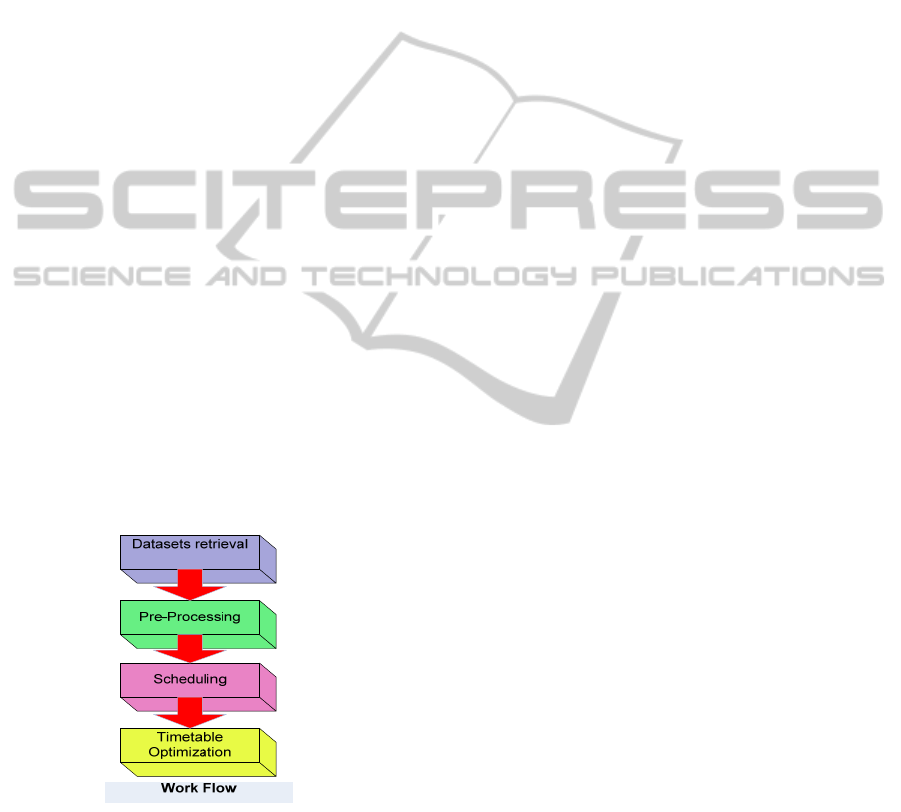
1.1 Overview of the Proposed Method
The steps of our proposed work in creating feasible
and quality examination schedules are datasets
retrieval, pre-processing, scheduling and lastly
timetable optimization as illustrated in Figure1.
Figure 1: The Work Flow in This Research.
Datasets retrieval can be defined as a task to
populate the four sets in the timetabling problem as
defined by (Burke et al., 2004). The 4 sets are the
times (T), resources (R), meetings (M) and
constraints (C). The task involves the process of
retrieving the datasets that are freely made available
to the public over the internet. In this research, we
have retrieved benchmark datasets that are widely
tested by many researchers from the University of
Nottingham and University of Toronto. These
benchmark datasets contain information or files
pertaining to students, exams, enrollments and other
data and constraints.
In the next step, which is the pre-processing
stage, a more meaningful information and higher
level data will be generated. This stage will be
underpinned by the methodology of Granular
Computing of generating semantically meaningful
information granules and their experimental
validation (Bargiela and Pedrycz, 2008). The
aggregated data will supply us with the important
information that is needed in order to create
timetables that are feasible which satisfy the basic
constraints. One example of the information
obtained from the pre-processing is the identification
of the clashing exams. By identifying this
information, later during the scheduling, we will be
able to schedule timetables that will fulfill the hard
constraint; for instance there should not be one
student having two exams simultaneously. In other
conventional approaches, this is not the case.
Without the pre-processing stage, the clashing
information is implicit in data, thus a lot of
permutations requiring a lot of time need to be done
in order to create a feasible timetable. This problem
can be avoided in our approach. Hence our approach
deals only with feasible solutions. The pre-
processing is explained in detail in (Rahim et al.,
2009).
Scheduling will be done next by using the
derived information from the previous process. The
scheduling is done by allocating exams with the
highest conflicts first to the available timeslots and
followed by exams with lower conflicts. Splitting
and merging of timeslots were done for exams in a
slot that can be reassigned to other slots consisting
non-conflicting exams. The allocation process has
been elaborated in detail in (Rahim et al., 2012). The
timetable generated at this stage is based on the pre-
processed data therefore it will always fulfill the
hard constraints.
The arrangements of the exams in the schedule
generated earlier might not fulfill many of the soft
constraints. Therefore, in order to improve the
quality of the exam schedules generated, we have
employed an optimization process. The optimization
consists of three procedures: i) Minimization of
Total Slot Conflicts, ii) Permutations of exams slots
and iii) Reassignments of exams between slots.
(Rahim et al., 2012). Please note that all the
ICORES2013-InternationalConferenceonOperationsResearchandEnterpriseSystems
242
optimization procedures mentioned here are done in
sequence but they are independent of each other.
In this paper, we will not be discussing about
these procedures in detail (it can be found in (Rahim
et al., 2012)), but will be looking at the possibility of
improving the quality of the schedules by
substituting the second step of optimization: the
permutations of exams slots which is a local search
procedure with a more effective procedure.
Realizing that our existing method (permutations
of exams slots), is a local search procedure, we
would like to incorporate a global search procedure
in order to see whether it could generate better
quality schedules. For this purpose, we have
implemented Genetic Algorithm (GA) to substitute
the permutations of exams slots in the optimization
process.
Genetic algorithm has been chosen as an
alternative approach to our implementation because
it has been proven a good way of producing good
examination timetables (Burke et al., 1994a); (Burke
et al., 1994b); (Gyori et al., 2001); (Ulker et al.,
2007). Besides, it has been mentioned that the
hybridisations of GA with some local search have
led to some success in this area. (Qu et al., 2009).
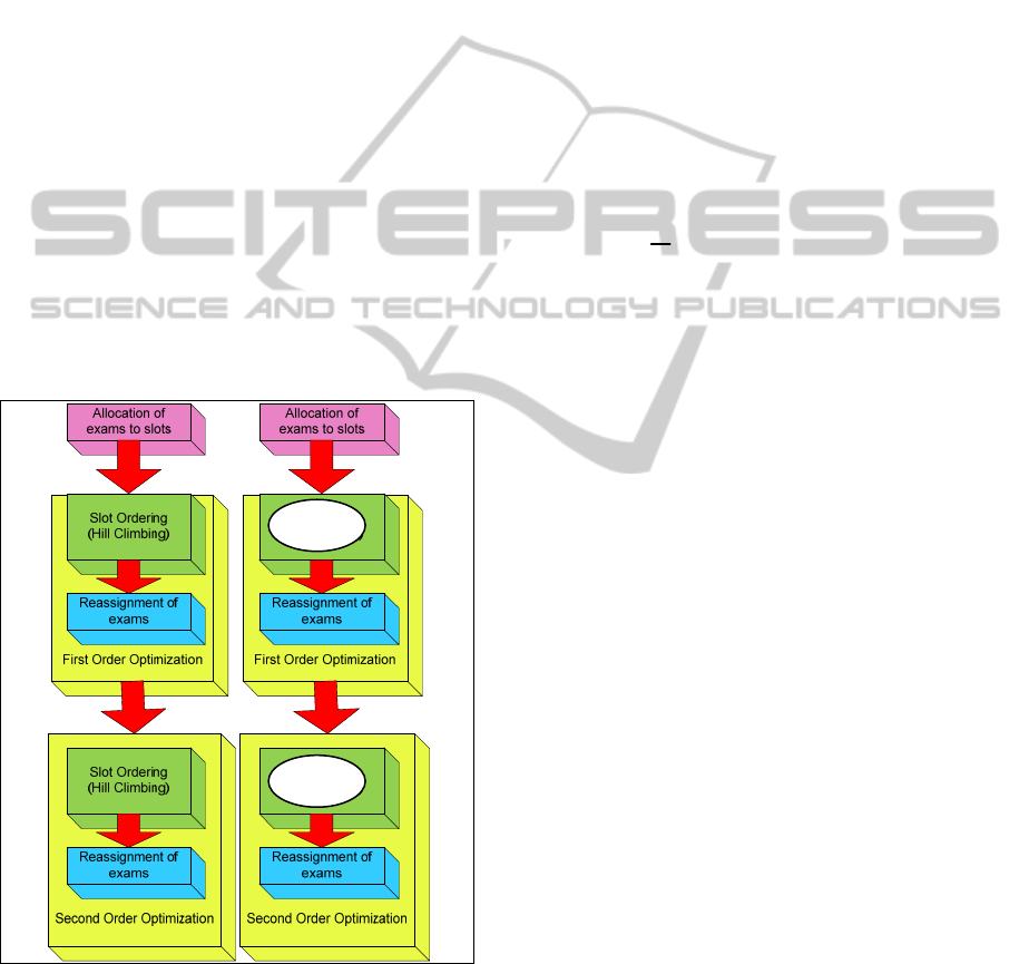
Figure 2: Scheduling and Optimization Steps Before and
After GA Substitution.
Above we presented the diagram (Figure 2) to
illustrate a summary of the work done in our
research (Rahim et al., 2012) which shows the
sequence of every process involve and the part that
will be substituted by GA. Please note that the whole
set of optimizations is done twice, therefore first and
second order optimization can be seen in the
diagram.
2 OPTIMIZATION METHODS
Normally, the cost of the initial timetables generated
by the allocation method mentioned earlier is a bit
high. This is because the ordering of exams to slots
might not satisfy many of soft constraints. An
example is the gap between conflicting exams is not
spaced out equally. The cost of the schedules is
measured by objective function proposed by Carter
(Carter et al., 1996) as below:
N
i
N
ij
ij
ws
T
11
pi| - pj|
1
(1)
where N is the number of exams, sij is the
number of students enrolled in both exam i and j, pj
is the time slot where exam j is scheduled, pi is the
time slot where exam i is scheduled and T is the total
number of students. According to this cost function,
a student taking two exams that are | pj - pi | slots
apart, where | pj - pi | ={1, 2, 3, 4, 5 }, leads to a cost
of 16, 8, 4, 2, and 1, respectively.
The lower the cost obtained, the better is the
quality of the schedule, since the gap between two
consecutive exams allows students to have
additional revision time.
2.1 Hill Climbing Optimization
In this optimization process, the permutations of
exam slots in the spread matrix (Rahim et al., 2009),
(Rahim et al., 2012) are done. This process involves
shuffling of slots or columns and so as block shifting
and swapping. The procedure started by reading a
spread matrix which is a matrix indicating how
many students taking an exam from slot ‘i’ and ‘j’.
The permutations in the spread matrix involved
swapping of slots and repetitions of block shifts.
Each slot will be swapped with another slot. This is
done by doing provisional swapping and the Carter
cost will be evaluated first. If the cost is reduced, the
swap will be remembered and the exam proximity
matrix will be updated according to this swap. Due
to this, we call this kind of optimization as a greedy
Hill Climbing (HC). The term greedy here refers to
the fact that we always take the best value whenever
GA
GA
HillClimbingversusGeneticAlgorithmOptimizationinSolvingtheExaminationTimetablingProblem
243
we found one. A number of repetitions of block shift
and swapping are done in order to ensure the search
space is explored in different directions so that
global optimum of the solutions can be found.
2.2 Genetic Algorithm Optimization
Genetic algorithm is a search heuristic that mimics
the process of natural evolution. It simulates the
inheritance of living beings and it is a widely used
method to solve optimization and search problems.
Genetic algorithm is a procedure used to find
approximate solutions to search problems by
mimicking the evolutionary biological process. It
operates on a population of solutions represented by
some encoding. Each member or unit of the
population consists of a number of genes,
representing a unit of information. This procedure
begins by creating an initial population (normally
randomly generated). Next the solution members are
evaluated by computing their fitness (or quality).
The selection procedure than reproduce more copies
of individuals with higher fitness values. The
selection procedure influences the search direction
towards promising areas. Genetic operators such as
crossover (mating two parents) and mutation (slight
random changes) are used to create new populations.
The important parameters include the population
size, crossover rate and mutation rate.
In our Genetic Algorithm implementation, we
defined the original parent as P0, which is a data
structure with the initial ordering of slots (1 …. N)
where N is the number of slots. GA creates a new
parent by moving position of the rows in blocks to
the new position, then appends it to array P. A
member of <npar> parents will be generated.
Generation of the new parents is just by shifting the
rows which in the end is the new representation of
the original parent with a magnitude maximum
distance of npar – 1. Therefore, if it is just a window
shift, there will be identical parents.
We then generated the new offspring. The
number of offspring to be generated is equals to npar
x npar -1. Each of the parents will be crossed over
with all other parents at a certain point R. The result
will be added to “o” which is the overall population.
The best parent will be automatically selected to
become one of the next generation parent. Then the
next best parent with the lowest cost will be
selected. The parent will be included in the next
population and the process continues for certain
number of generations.
3 COMPUTATIONAL RESULTS
AND DISCUSSION
The experiment in this work was performed on all
13 datasets in the Toronto benchmark repository
[ftp://ftp.mie.utoronto.ca/pub/carter/testprob] and
also on the Nottingham dataset
[http://www.cs.nott.ac.uk/~rxq/files/Nott.zip]. For
the sake of comparability with other studies in the
literature, these problems are considered here as an
uncapacitated scheduling problem. Uncapacitated
means the total room capacity in each time slot is
not considered.
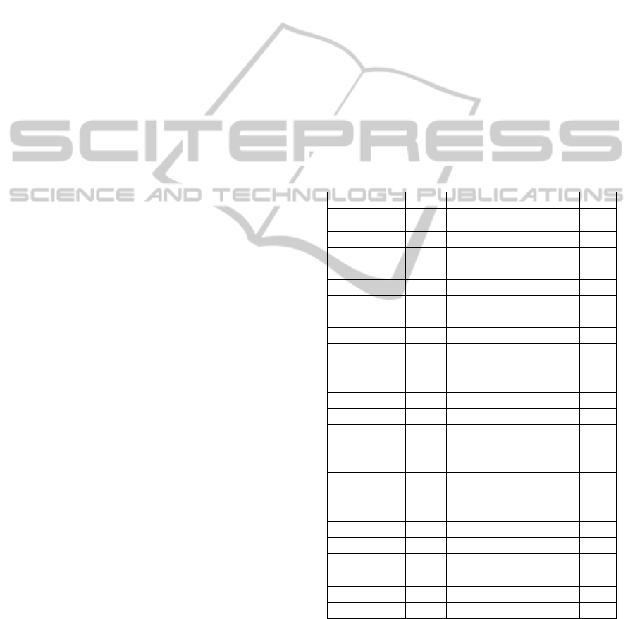
The characteristics of all the datasets are listed in
Table 1. For the Toronto datasets, based on the
survey made by (Qu et al., 2009), 8 out of 13
problem instances exist in 2 versions. We will use
version I of the datasets which are extensively tested
by other researchers.
Table 1: The characteristics of the Datasets.
(a) (b) (c) (d) (e) (f)
nott (a/b) 800 7896 33997 23 0.03
car-s-91 (I) 682 16925 56877 35 0.13
car-s-91 (II) 682 16925 56242/
56877
35 0.13
car-f-92 (I) 543 18419 55522 32 0.14
car-f-92 (II) 543 18419 55189/
55522
32 0.14
ear-f-83(I) 190 1125 8109 24 0.27
ear-f-83(II) 189 1108 8014 24 0.27
hec-s-92(I) 81 2823 10632 18 0.42
hec-s-92(II) 80 2823 10625 18 0.42
kfu-s-93 461 5349 25113 20 0.06
lse-f-91 381 2726 10918 18 0.06
pur-s-93 (I) 2419 30029 120681 42 0.03
pur-s-93 (II) 2419 30029 120686/
120681
42 0.03
rye-f-92 486 11483 45051 23 0.07
sta-f-83(I) 139 611 5751 13 0.14
sta-f-83(II) 138 549 5689 35 0.14
tre-s-92 261 4360 14901 23 0.18
uta-s-92(I) 622 21266 58979 35 0.13
uta-s-92(II) 638 21329 59144 35 0.13
ute-s-92 184 2749 11793 10 0.08
yor-f-83 (I) 181 941 6034 21 0.29
yor-f-83 (II) 180 919 6012 21 0.29
(a)Name of Dataset; (b) No of Exams; (c) No of Students;
(d) No of Enrollments; (e) Required No of Slots; (f)
Conflict Density.
We have shown the results obtained by using
Hill Climbing and Genetic Algorithm optimization
ICORES2013-InternationalConferenceonOperationsResearchandEnterpriseSystems
244

on the initial feasible schedule generated by our
allocation method before performing other
optimization process (Rahim et al., 2012) in Table 2
to Table 15. For the Hill Climbing, we recorded the
worse and the best cost during the process
(permutations of slots), and for the Genetic
Algorithm, we presented the cost produced after
Generation 1 (Gen 1) and Generation 15 (Gen 15).
The best cost produced for each type of
optimization is accepted and the ordering of slots
were rearranged accordingly before doing further
optimization : reassignment of exams between slots
(Rahim et al., 2012) and later repeating the whole set
of the optimization process until there is no
improvement in the schedule cost (Rahim et al.,
2012). The accepted cost together with the CPU time
taken for each process can be seen in these tables.
Table 2: Results obtained by optimization for nott.
Dataset
/
Initial
Cost
Cost
Accepted
Cost
CPU Time
(seconds)
Hill Climbing
Worse
cost
Best
cost
nott
31.95 10.94
10.94 187.27
38.99
Genetic Algorithm
Gen 1 Gen 15
28.03 14.74 14.74 3.39
Table 3: Results obtained by optimization for car-f-92(I).
Dataset
/
Initial
Cost
Cost
Accepted
Cost
CPU Time
(seconds)
Hill Climbing
Worse
cost
Best
cost
car-f-92
(I)
8.89 5.36
5.36 268.97
9.43
Genetic Algorithm
Gen 1 Gen 15
8.07 6.68 6.68 5.11
Table 4: Results obtained by optimization for car-s-91(I).
Dataset
/
Initial
Cost
Cost
Accepted
Cost
CPU Time
(seconds)
Hill Climbing
Worse
cost
Best
cost
car-s-91
(I) 10.43 6.26
6.26 351.39
11.77
Genetic Algorithm
Gen 1 Gen 15
9.37 8.10 8.10 5.99
Table 5: Results obtained by optimization for ear-f-83(I).
Dataset
/
Initial
Cost
Cost
Accepted
Cost
CPU Time
(seconds)
Hill Climbing
Worse
cost
Best
cost
ear-f-83
(I)
62.57 40.45 40.45 136.77
72.69
Genetic Algorithm
Gen 1 Gen 15
53.51 48.99 48.99 1.78
Table 6: Results obtained by optimization for hec-s-92(I).
Dataset
/
Initial
Cost
Cost
Accepted
Cost
CPU Time
(seconds)
Hill Climbing
Worse
cost
Best
cost
hec-s-92
(I)
22.55 12.52
12.52 27.52
22.83
Genetic Algorithm
Gen 1 Gen 15
19.39 14.14 14.14 2.30
HillClimbingversusGeneticAlgorithmOptimizationinSolvingtheExaminationTimetablingProblem
245
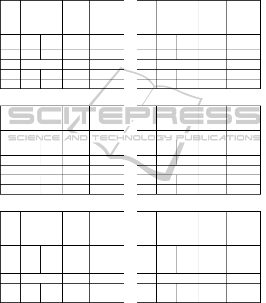
Table 7: Results obtained by optimization for kfu-s-93.
Dataset
/
Initial
Cost
Cost
Accepted
Cost
CPU Time
(seconds)
Hill Climbing
Worse
cost
Best
cost
kfu-s-93 29.89 16.06 16.06 40.36
37.79
Genetic Algorithm
Gen 1 Gen 15
26.81 20.06 20.06 2.48
Table 8: Results obtained by optimization for lse-f-91.
Dataset
/
Initial
Cost
Cost
Accepted
Cost
CPU Time
(seconds)
Hill Climbing
Worse
cost
Best
cost
lse-f-91 22.42 14.63 14.63 26.59
23.77
Genetic Algorithm
Gen 1 Gen 15
19.40 17.20 17.20 2.25
Table 9: Results obtained by optimization pur-s-93(I).
Dataset
/
Initial
Cost
Cost
Accepted
Cost
CPU Time
(seconds)
Hill Climbing
Worse
cost
Best
cost
pur-s-93
(I)
14.27 6.69 6.69 321.05
14.91
Genetic Algorithm
Gen 1 Gen 15
11.94 8.47 8.47 7.97
Table 10: Results obtained by optimization for rye-f-92.
Dataset
/
Initial
Cost
Cost
Accepted
Cost
CPU Time
(seconds)
Hill Climbing
Worse
cost
Best
cost
rye-f-92 28.55 12.68 12.68 73.17
31.50
Genetic Algorithm
Gen 1 Gen 15
19.04 16.46 16.46 3.25
Table 11: Results obtained by optimization sta-f-83(I).
Dataset
/
Initial
Cost
Cost
Accepted
Cost
CPU Time
(seconds)
Hill Climbing
Worse
cost
Best
cost
sta-f-83 193.47 158.43 158.43 10.28
201.95
Genetic Algorithm
Gen 1 Gen 15
172.80 163.12 163.12 0.52
Table 12: Results obtained by optimization for tre-s-92.
Dataset
/
Initial
Cost
Cost
Accepted
Cost
CPU Time
(seconds)
Hill Climbing
Worse
cost
Best
cost
tre-s-92
13.25 9.84 9.84 66.34
14.81
Genetic Algorithm
Gen 1 Gen 15
12.76 11.70 11.70 3.17
ICORES2013-InternationalConferenceonOperationsResearchandEnterpriseSystems
246
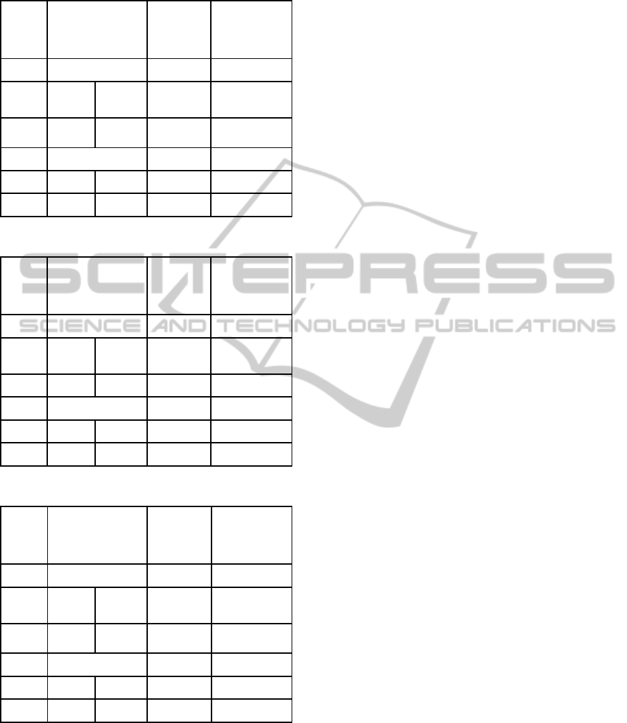
Table 13: Results obtained by optimization utas-s-92(I).
Dataset
/
Initial
Cost
Cost
Accepted
Cost
CPU Time
(seconds)
Hill Climbing
Worse
cost
Best
cost
uta-s-92
(I)
6.59 4.23
4.23 455.94
7.30
Genetic Algorithm
Gen 1 Gen 15
6.19 5.22 5.22 6.54
Table 14: Results obtained by optimization for ute-s-92.
Dataset
/
Initial
Cost
Cost
Accepted
Cost
CPU Time
(seconds)
Hill Climbing
Worse
cost
Best
cost
ute-s-92 43.25 31.79 31.79 2.91
56.97
Genetic Algorithm
Gen 1 Gen 15
35.77 32.96 32.96 1.30
Table 15: Results obtained by optimization for yor-f-83(I).
Dataset
/
Initial
Cost
Cost
Accepted
Cost
CPU Time
(seconds)
Hill Climbing
Worse
cost
Best
cost
yor-f-83
(I)
56.31 43.36
43.36 46.99
59.04
Genetic Algorithm
Gen 1 Gen 15
50.77 47.50 47.50 0.75
Based on the results presented in Table 2 to
Table 15, it can be seen clearly that our proposed
greedy Hill Climbing (HC) method has
outperformed GA in all cases during the
optimization when tested on the benchmark datasets.
All the results produced by GA for all the datasets
after generation 15 (Gen 15) were not able to
outperform results produced by HC.
It is worth highlighting here that the cost
obtained by GA for all datasets at generation 1 (Gen
1) are quite encouraging, where they are much lower
than the worse cost obtained by HC. However, all of
them failed to outperform the cost obtained by HC
after generation 15 (Gen 15).
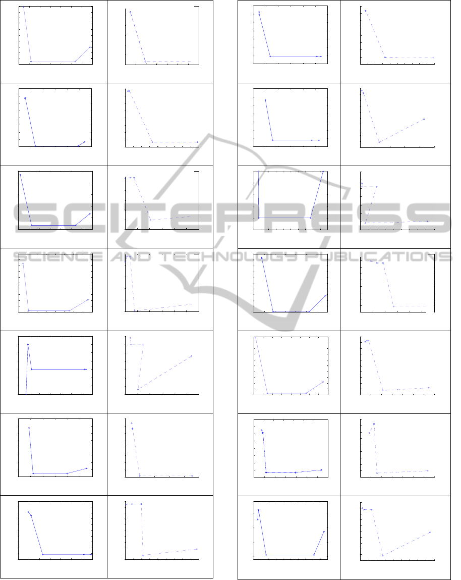
Using the data gathered from the experiments on
all the datasets, we have plotted graphs for the cost
(1) versus the Total Slot Conflicts as in Figure 3 and
Figure 4. Figure 3 and 4 show the graphs for the
cost(1) versus the Total Slot Conflicts plotted for all
benchmark datasets tested. Diagram (a1), (b1), (c1),
(d1), ….. (n1) are the graphs (line-graphs) when HC
optimization used where as diagram (a2), (b2), (c2),
(d2),…… (n2) are the graphs (dotted-graphs) plotted
when GA optimization used. The diagrams in these
figures are arranged according to the sequence of
datasets from Table 2 to Table 15.
Based on the graphs presented, the horizontal
line constructed from the second data point to third
data point in diagram (a1) to (n1) is due to reduction
of cost via permutations of exams slots (greedy HC)
which did not involve any augmentation of total
slots conflicts (Rahim et al., 2012). The dotted line
from the first data point to the second data point in
each diagram (a2) to (n2) is constructed based on the
GA optimization discussed earlier in this paper.
The dotted lines in this stage showed that a
significant reduction in terms of the initial cost has
been achieved by performing the GA optimization.
These lines also showed that our GA implementation
managed to substitute the HC implementation and
was incorporated successfully in the whole set of our
optimization process. (Rahim et al., 2012).
One of the obvious thing that can be seen in the
graphs is that the line constructed by GA
optimization is not always horizontal. This is
because, the crossover and mutation of exam slots in
the GA optimization process had changed the
assignments of some exams to slots to ensure the
feasibility of the schedules, thus changing the
existing number of total slots conflicts. This is not
the case duirng HC optimization where by the total
exam-slot conflict does not change because the
individual exams to slots remain as before
permutations. (Rahim et al., 2012).
An interesting point to note is the computational
time taken to execute both methods. Even though
GA did not surpass HC in all cases, however the
time taken to execute the process was incredibly fast
compared to our HC implementation. We have
managed to implement a simple, straightforward and
quite effective GA which consumed very little
HillClimbingversusGeneticAlgorithmOptimizationinSolvingtheExaminationTimetablingProblem
247
5 10 15 20 25 30 35 40
8
8.2
8.4
8.6
8.8
9
9.2
9.4
9.6
9.8
10
Tot al s lot conf lict * 1000
Carter cost
(a1)
5 10 15 20 25 30 35 40
7.5
8
8.5
9
9.5
10
10.5
Carter cost
Total slot conflic t * 1000
(a2)
4 5 6 7 8 9 10
12.2
12.4
12.6
12.8
13
13.2
13.4
13.6
13.8
Carter c ost
Total slot conflic t * 1000
(b1)
5 5.5 6 6.5 7 7.5 8 8.5 9 9.5
12.2
12.4
12.6
12.8
13
13.2
13.4
13.6
13.8
Carter cost
Total sl ot confl ict * 1000
(b2)
5 6 7 8 9 10 11 12
16.5
17
17.5
18
18.5
19
Carter cost
Total slot c onflict * 1000
(c1)
6 7 8 9 10 11 12
16.5
17
17.5
18
18.5
19
19.5
Carter cost
Tota l s lot conf li ct * 1000
(c2)
35 40 45 50 55 60 65 70 75
3.54
3.56
3.58
3.6
3.62
3.64
3.66
3.68
3.7
3.72
3.74
Carter cost
Total s lot confl ict * 1000
(d1)
45 50 55 60 65 70 75
3.55
3.6
3.65
3.7
3.75
3.8
Carter cost
Total slot c onflict * 1000
(d2)
10 12 14 16 18 20 22 24
1.26
1.26 1
1.26 2
1.26 3
1.26 4
1.26 5
1.26 6
1.26 7
Carter cost
Total slot c onflict * 1000
(e1)
12 14 16 18 20 22 24
1.24
1.245
1.25
1.255
1.26
1.265
1.27
1.275
Carter cost
Total sl ot confl ict * 1000
(e2)
10 15 20 25 30 35 40
4.5
4.6
4.7
4.8
4.9
5
5.1
5.2
5.3
Carter cost
Total slot c onflict * 1000
(f1)
15 20 25 30 35 40
4.6
4.7
4.8
4.9
5
5.1
5.2
5.3
5.4
Carter cost
Total sl ot confl ict * 1000
(f2)
10 12 14 16 18 20 22 24
3.7
3.75
3.8
3.85
3.9
3.95
4
4.05
4.1
4.15
4.2
Carter cost
Total slot c onflict * 1000
(g1)
15 16 17 18 19 20 21 22 23 24
3.65
3.7
3.75
3.8
3.85
3.9
3.95
4
4.05
4.1
4.15
Carter cost
Total s lot confl ict * 1000
(g2)
Figure 3: Cost (1) vs. the Total Slot Conflicts for
Benchmark Datasets (Using Hill Climbing (a1)-(g1) vs
Genetic Algorithm (a2)-(g2)).
4 6 8 10 12 14 16
48
50
52
54
56
58
60
62
Carter cost
Total slot c onflict * 1000
(h1)
5 6 7 8 9 10 11 12 13 14 15
48
50
52
54
56
58
60
62
64
Carter cost
Total s lot confl ict * 1000
(h2)
5 10 15 20 25 30 35
7.1
7.2
7.3
7.4
7.5
7.6
7.7
7.8
Carter cost
Total slot c onflict * 1000
(i1)
10 15 20 25 30 35
6.7
6.8
6.9
7
7.1
7.2
7.3
7.4
7.5
7.6
7.7
Total s lot c onflic t * 1000
Carter cost
(i2)
155 160 16 5 170 175 180 185 190 195 200 205
1.5045
1.50 5
1.5055
1.50 6
1.5065
1.50 7
Carter cost
Total slot c onflict * 1000
(j1)
160 165 170 175 180 185 190 195 200 205
1.5
1.505
1.51
1.515
1.52
1.525
1.53
1.535
Carter cost
Total slot confli ct * 1000
(j2)
8 9 10 11 12 13 14 15
4.25
4.3
4.35
4.4
4.45
4.5
4.55
4.6
4.65
4.7
4.75
Carter cost
Total slot c onflict * 1000
(k1)
9 10 11 12 13 14 15
4.35
4.4
4.45
4.5
4.55
4.6
4.65
4.7
4.75
4.8
Carter cost
Total slot c onflict * 1000
(k2)
3.5 4 4.5 5 5. 5 6 6.5 7 7. 5
14.8
15
15.2
15.4
15.6
15.8
16
16.2
16.4
16.6
16.8
Carter cost
Total slot c onflict * 1000
(l1)
4 4.5 5 5. 5 6 6.5 7 7. 5
15
15.2
15.4
15.6
15.8
16
16.2
16.4
16.6
16.8
17
Carter cost
Total s lot confl ict * 1000
(l2)
25 30 35 40 45 50 55 60
1.14
1.16
1.18
1.2
1.22
1.24
1.26
Carter cost
Total s lot confl ict * 1000
(m1)
25 30 35 40 45 50 55 60
1.14
1.16
1.18
1.2
1.22
1.24
1.26
1.28
1.3
Carter cost
Total sl ot confl ict * 1000
(m2)
40 42 44 46 48 50 52 54 56 58 60
3.25
3.3
3.35
3.4
Carter cost
Total slot c onflict * 1000
(n1)
42 44 46 48 50 52 54 56 58 60
3.24
3.26
3.28
3.3
3.32
3.34
3.36
3.38
3.4
3.42
3.44
Carter cost
Total s lot confl ict * 1000
(n2)
Figure 4: Cost (1) vs. the Total Slot Conflicts for
Benchmark Datasets (Using Hill Climbing (h1)-(n1) vs
Genetic Algorithm (h2)-(n2)).
ICORES2013-InternationalConferenceonOperationsResearchandEnterpriseSystems
248
amount of time to improve the initial feasible
schedule, although majority researchers claimed that
the GA took a very huge time in order to solve the
scheduling problem (for example claimed by
(Abramson, 1992)).
This advantage (minimal time requirement)
could offer even more advantage, because based on
the results presented earlier we can predict that
addition to the number of iterations or generations
(with the aim to generate better offsprings) to the
GA execution will add only little more
computational time that would definitely be very
acceptable.
However, unfortunately this is not the case. The
increase in the number of generations has not given
any benefit to the reduction of the cost of the exam
schedule generated. We have experimented 15
generations, but it seems like the highest number of
generations that manage to reduce the cost is
generation 12 (car-f-92(I)). Recall that we have
mentioned previously, a second round of
optimization was done in order to test whether it
could reduce the cost further. Therefore, after
performing reassignment of exams on the schedules
obtained by the GA optimization (Rahim et al.,
2012), we have repeated the GA optimization one
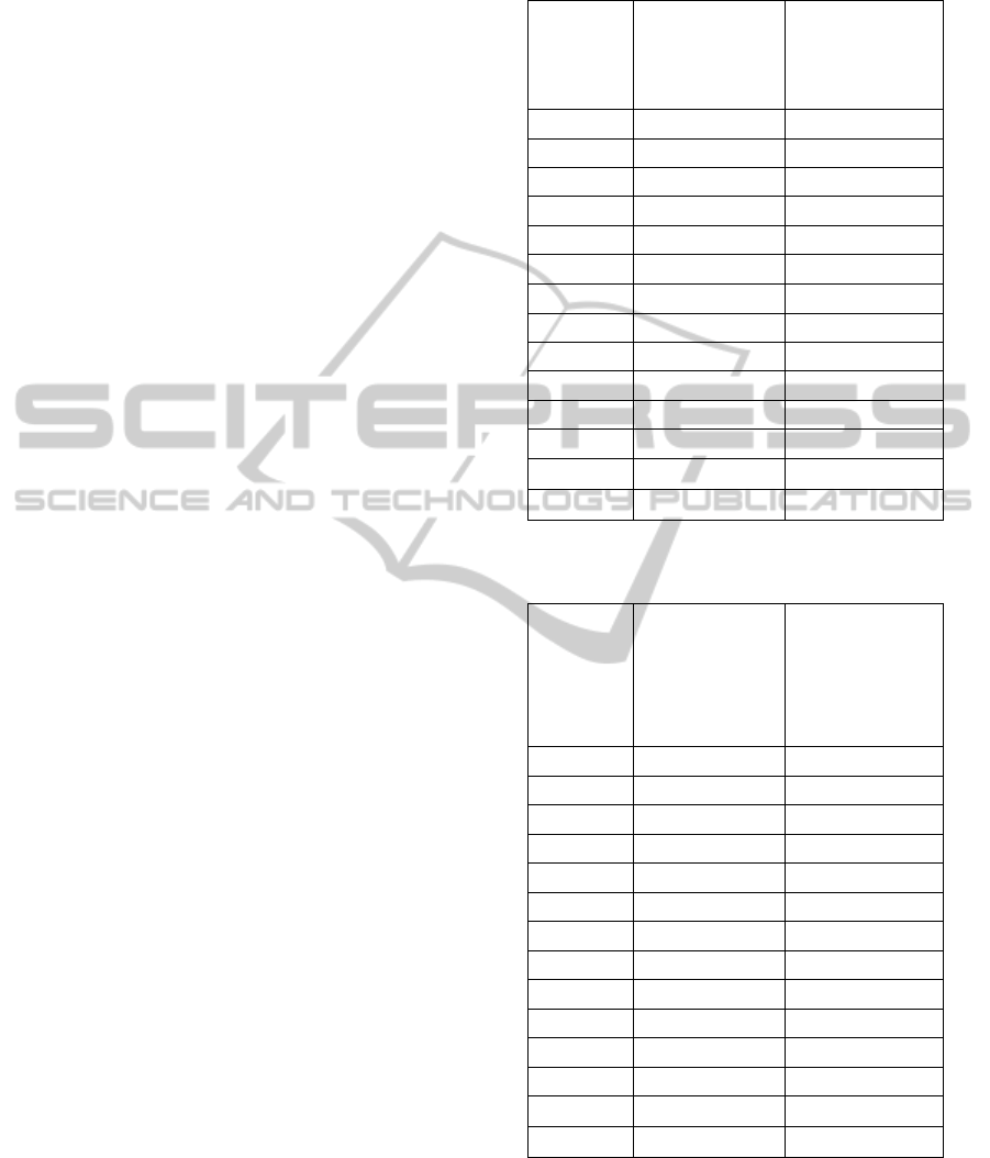
more time. As can be seen in Table 16, the highest
number of generations that could reduce the
schedule cost is generation 11 (rye-f-92) even
though 15 generations was tested.
The second round has improved the cost(1) for
most of the datasets (exceptional for nott, carf92,
kfus93, purs93, and utes9) and this is illustrated in
diagram (a2) until (n2) by the third data point to the
fourth data point.
The final results obtained by HC and GA
methods which later were further improved by
reassignments of exams (Rahim et al., 2012) were
compared and can be found in Table 17. It can be
seen clearly that HC outperforms GA in all cases,
though the execution time recorded was a bit high in
comparison to GA, but the amount of time taken was
still reasonable which is only a few hundreds
seconds CPU time.
4 CONCLUSIONS
In conclusion, it is shown that GA has been proven
to be a good method to reduce the cost of the initial
feasible timetable. With a robust implementation, it
managed to explore the search space efficiently and
produce good quality timetable with an incredibly
fast execution time.
Table 16: Number of Generations That Could Improve the
Schedule Cost During GA Optimization.
Dataset
First Order
Optimization:
Cost Improved
Until Iteration
Second Order
Optimization:
Cost Improved
Until Iteration
notts 7 0
carf92 12 0
cars91 9 2
earf83 7 6
hecs92 6 7
kfus93 10 0
lsef91 8 4
purs93 11 0
ryef92 8 11
staf83 6 4
tres92 8 5
utas92 10 4
utes92 3 0
yorf83 6 3
Table 17: Final Cost Produced Using HC versus GA
Optimization.
Dataset
Final Cost
Produced after All
Optimizations
Processes For HC
(Rahim et al.,
2012)
Final Cost
Produced after All
Optimizations
Processes For GA
notts 7.34 7.62
carf92 4.49 5.18
cars91 5.19 6.03
earf83 37.57 45.08
hecs92 11.47 12.90
kfus93 14.36 17.27
lsef91 11.90 15.11
purs93 4.88 5.57
ryef92 9.8 10.63
staf83 158.25 161.13
tres92 8.74 9.86
utas92 3.58 4.01
utes92 27.37 29.35
yorf83 41.10 43.52
However, the good cost obtained through the
experiment with GA did not manage to outperform
the results obtained by utilizing our proposed greedy
HC. Although the computational time taken by GA
execution is very much lower than HC, but an
additional reasonable amount of time taken to obtain
HillClimbingversusGeneticAlgorithmOptimizationinSolvingtheExaminationTimetablingProblem
249

qood quality schedules is considered very worth
while. Since HC managed to improve the initial
feasible schedule without fail for all datasets and
always surpass the GA results, therefore it is
suggested that the proposed HC is incorporated and
used in our whole set of optimization process.
Through the findings of this research, it makes it
more understandable to us the claim made by (Ross
et al., 1998) that sometimes GA is not a very good
approach in solving problems.
In the future work, we will try to implement
other types of search procedures to be incorporated
with our proposed method for example the Late
Acceptance Hill Climbing method which has been
proven to be very effective in producing
encouraging results to the examination scheduling
problem. (Bykov et al., 2008); (Bykov et al., 2009).
REFERENCES
A. J. Abramson D. 1992. A parallel genetic algorithm for
solving the school timetabling problem.
Asmuni H., E. K. Burke, J. M. Garibaldi, and Barry
McCollum. 2005. Fuzzy Multiple Heuristic Orderings
for Examination Timetabling. In E. K. Burke and M.
Trick, editors, Practice and Theory of Automated
Timetabling V (PATAT 2004, Pittsburg USA, August
2004, Selected Revised Papers), volume 3616 of
Lecture Notes in Computer Science, pages 334–353,
Berlin, 2005.Springer.
Asmuni H, E. K. Burke, J. M. Garibaldi, B. McCollum
and A. J. Parkes. 2009. An investigation of fuzzy
multiple heuristic orderings in the construction of
university examination timetables. Comput. Oper.
Res.,vol. 36, pp. 981-1001, 2009.
Bargiela, A. Pedrycz, W., 2008. Toward a theory of
Granular Computing for human-centred information
processing. IEEE Trans. on Fuzzy Systems, vol. 16, 2,
2008, 320-330, doi:10.1109/TFUZZ.2007.905912.
Bykov Y., Burke E. K. 2008. A late acceptance strategy in
hill-climbing for exam timetabling problems. PATAT
2008 Conference. Montreal, Canada.
Bykov Y., E. Ozcan, M. Birben. 2009. Examination
timetabling using late acceptance hyper-heuristics.
IEEE Congress on Evolutionary Computation.
Burke E. K., Elliman D. G., and Weare R. F. 1994a. A
Genetic Algorithm for University Timetabling. AISB
Workshop on Evolutionary Computing, University of
Leeds, UK.
Burke E. K., Elliman D. G., and Weare R. F. 1994b. A
Genetic Algorithm Based University Timetabling
System. AISB Workshop on Evolutionary Computing,
University of Leeds, UK.
Burke E. K., Bykov Y., Newall J. and Petrovic S. 2004. A
Time-Predefined Local Search Approach to Exam
Timetabling Problems. IIE Transactions on Operations
Engineering, 36(6) 509-528.
Burke E. K., Pham N, Yellen J. 2010c. Linear
Combinations of Heuristics for Examination
Timetabling. Annals of Operations Research DOI
10.1007/s10479-011-0854-y.
Carter M. and Laporte G. 1995. Recent developments in
practical examination timetabling. Lecture Notes in
Comput. Sci., vol 1153, pp.1-21, 1996 [Practice and
Theory of Automated Timetabling I, 1995].
Carter M., Laporte G. and Lee S. 1996. Examination
Timetabling: Algorithmic Strategies and Applications.
Journal of Operations Research Society, 47 373-383.
Dowsland K. A. and Thompson J. 2005. Ant colony
optimization for the examination scheduling problem.
Journal of Operational Research Society, 56: 426-438.
Gueret,. Narendra Jussien, Patrice Boizumault, Christian
Prins. 1995. Building University Timetables Using
Constraint Logic Programming. First International
Conference on the Practice and Theory of Automated
Timetabling, PATAT’ 95, pp. 393-408, Edinburgh.
Gyori S., Z. Petres, and A. Varkonyi-Koczy. Genetic
Algorithms in Timetabling. A New Approach. 2001.
Budapest University of Technology and Economics,
Department of Measurement and Information Systems.
Qu. R, Burke E. K., B. McCollum, L. T. G. Merlot, and S.
Y. Lee. 2009. A Survey of Search Methodologies and
Automated System Development for Examination
Timetabling. Journal of Scheduling, 12(1): 55-89,
2009. doi: 10.1007/s10951-008-0077-5.
Rahim, S. K. N. A., Bargiela, A., & Qu, R. 2009. Granular
Modelling Of Exam To Slot Allocation. ECMS 2009
Proceedings edited by J. Otamendi, A. Bargiela, J. L.
Montes, L. M. Doncel Pedrera (pp. 861-866).
European Council for Modeling and Simulation.
doi:10.7148/2009-0861-0866.
Rahim, S. K. N. A., Bargiela, A., & Qu, R. 2012. Domain
Transformation Approach to Deterministic
Optimization of Examination Timetables. Accepted
for publication in Artificial Intelligence Research
(AIR) Journal. Sciedu Press.
Ross P., Hart E. and Corne D. 1998. Some observations
about GA-based exam timetabling. In: E.K. Burke and
M.W. Carter (eds) (1998). Practice and Theory of
Automated Timetabling: Selected Papers from the 2nd
International Conference. Springer Lecture Notes in
Computer Science, vol. 1408. 115-129.
Taufiq Abdul Gani, Ahamad Tajudin Khader and Rahmat
Budiarto. 2004. Optimizing Examination Timetabling
using a Hybrid Evolution Strategies. IN: Proceedings
of the Second International Conference on
Autonomous Robots and Agents (ICARA 2004), 13-
15 December 2004, Palmerston North, New Zealand,
pp. 345-349.
Ulker O., Ozcan E. and E. E. Korkmaz. 2007. Linear
linkage encoding in grouping problems: applications
on graph coloring and timetabling. In: E.K. Burke and
H. Rudova (eds) (2007) Practice and Theory of
Automated Timetabling: Selected Papers from the 6th
International Conference. Springer Lecture Notes in
Computer Science, vol. 3867, 347-363.
ICORES2013-InternationalConferenceonOperationsResearchandEnterpriseSystems
250
