Lagrangian Road Pricing
Vianney Boeuf
1
and S
´
ebastien Blandin
2
1
´
Ecole Polytechnique Paristech, Paris, France
2
IBM Research Collaboratory, Singapore, Singapore
Keywords:
Road Pricing, Traffic Assignement, User Equilibrium, Congestion Toll Pricing, Multicommodity Flows.
Abstract:
We consider the problem of trajectory-based road pricing with the objective of reducing congestion on a road
network. It is well-known that traffic conditions resulting from typical non-cooperative behavior of selfish
drivers do not minimize total travel time spent on the road network. In the context of real-time GPS data
collection from all vehicles, drivers can be charged differently based on their origin and destination, and
according to the path they take from that origin to that destination. In this work, we propose a new formulation
of the set of multi-commodity prices based on a price potential, and describe an efficient algorithm to construct
such multi-commodity prices. We provide an analysis of the subset of valid prices satisfying several specific
user-driven constraints. The numerical performances of the method proposed are assessed on a benchmark
network, and the social benefits resulting from the commodity-based potential pricing scheme introduced in
this article are discussed.
1 INTRODUCTION
Congestion pricing, which dates back to 1969 with
the work of (Vickrey, 1969), is motivated by the fun-
damental difference existing between the natural state
of traffic, typically assumed to be a user equilibrium
or Wardrop equilibrium, and the best possible alloca-
tion of traffic, or “social optimum”. The difference
between these two states of traffic has been called
the “price of anarchy” (Papadimitriou, 2001). A user
equilibrium can be arbitrarily far from the social opti-
mum, as soon as instances of Braess paradox (Braess,
1968) exist in the network.
Pricing schemes aim at designing a tolled user
equilibrium coinciding with the social optimum of
the network. A basic solution consists of “internaliz-
ing externalities” by charging users with the marginal
costs they occur to the network (Pigou, 1920). How-
ever, more specific operator or user-driven constraints
such as profit maximization, or fairness guarantees,
have historically motivated the search for other pric-
ing schemes.
The recent improvement in real-time positioning
capabilities using GPS devices (Mobile Millenium,
2008) creates new possibilities and challenges for
congestion pricing. Charging users based on their
path properties, and not only at sparse locations on
the road network, is now technically feasible.
In this article, we consider the problem of char-
acterizing feasible Lagrangian (trajectory-based) toll
sets achieving a given flow allocation on the network.
We allow different prices for different origin - desti-
nation pairs (multi-commodity pricing), and provide
an extension of the toll set formulation first proposed
by (Hearn and Ramana, 1998), as the translation of
the set of prices generated by a potential on the nodes
of the network. In particular, we show that the set of
feasible prices obtained for trajectory-based pricing is
convex (Boyd and Vandenberghe, 2004).
We provide an algorithm to construct a pricing
scheme for different strategies (Hearn and Ramana,
1998) and assess the performance of our pricing
schemes against benchmark pricing algorithms. Nu-
merical simulations and performance analysis are per-
formed in Python using a convex optimization library
(Dahl and Vandenberghe, 2008).
The rest of the article is organized as follows.
In section 2, we introduce notations. In section 3,
we present our main results, on the characterization
and properties of a commodity-based potential pric-
ing scheme. Section 4 presents a numerical study of
the problem. Finally, section 5 provides concluding
remarks and discusses extensions to this work.
144
Boeuf V. and Blandin S..
Lagrangian Road Pricing.
DOI: 10.5220/0004287102920297
In Proceedings of the 2nd International Conference on Operations Research and Enterprise Systems (ICORES-2013), pages 292-297
ISBN: 978-989-8565-40-2
Copyright
c
 2013 SCITEPRESS (Science and Technology Publications, Lda.)

2 PRELIMINARIES
In this section, we introduce the notations and prelim-
inary results leading to our problem formulation and
the main results of the following section.
2.1 Notations
Let graph G = (N , A) represent the road network,
and K denote the set of origin-destination (OD) pairs
(if k ∈ K, k = (p, q), p, q ∈ N ), and (d
k
)
k∈K
the travel
demand for pair k. Several representations of the traf-
fic flow on the network can be used.
Path Flows. For k = (p, q) ∈ K, let R
k
denote the
set of directed acyclic paths connecting the origin p
with the destination q, and let R := ∪
k∈K
R
k
. h =
(h
r
)
r∈R
is the path flow. h is feasible if it is positive
and satisfies demand. H is the set of feasible path
flows.
∑
r∈R
k
h
r
= d
k
∀k ∈ K and 0 ≤ h
r
∀r ∈ R . (1)
If we note Γ the OD-paths incidence matrix, then
equation (1) can be written as :
Γ
T
h = d and 0 ≤ h.
Let h ∈ H be a feasible flow. We note R
k,h−eff
=
{r ∈ R
k
|h
r
> 0} , and R
h−eff
= ∪
k∈K
R
k,h−eff
the set
of paths for which the flow h is positive.
We note R
i, j
the set of paths from i to j.
Commodity Arc Flows. Let w
k
a
be the flow of ve-
hicles from OD pair k = (p, q) going through arc a,
and w
k
the vector of arc flows for OD pair k. In
this context, k is a commodity and w
k
an OD-flow or
commodity-flow. w
k
a
=
∑
r∈R
k
,a∈r
h
r
.
We note E the node-arc incidence matrix, and for
k = (p, q), i
k
∈ ℜ
|N |
the node-OD incidence vector,
i.e. the vector such that for n ∈ N , i
k
n
= +1 if n = q,
i
k
n
= −1 if n = p and 0 otherwise. w is feasible if and
only if:
Ew
k
= d
k
i
k
∀k ∈ K and 0 ≤ w
k
∀k ∈ K. (2)
W is the set of feasible commodity flows.
We denote by
˜
E the matrix



E 0 .. 0
0 E .. 0
...
0 0 .. E



such
that
˜
Ew = (d
k
i
k
)
k∈K
.
Arc Flows. An aggregate flow f = ( f
a
)
a∈A
is de-
fined on each arc a as the total traffic flow on each arc
of the network. It can be computed from h or w:
f
a
=
∑
r∈R ,a∈r
h
r
∀a ∈ A or f = Λh (3)
f
a
=
∑
k
w
k
a
∀a ∈ A or f =
∑
k
w
k
(4)
where Λ is the arc-path incidence matrix (Λ)
a,r
=
δ
a∈r
.
A flow f is feasible if it is the sum of feasible com-
modity flows or of a feasible path flow. F is the set of
feasible flows f .
We call the three flows f , w
k
, k ∈ K, h equivalent
if f and w can be computed from h and if one of the
three given flows is feasible.
Finally, we use the generic notation v = (v
i
)
i∈I
to
denote the arc, path or commodity formulation. We
denote by V the set of feasible flows v, n = |I| the
number of traces on which v is defined, A the matrix
of linear constraints (
˜
E if v = w and Γ
T
if v = h) and
p the number of rows of A (resp. |N | and |K|).
If v denotes a flow with only one OD pair,
R
v−eff
i, j
= {r ∈ R
i, j
|h
r
> 0} where h is the path flow
associated to v.
2.2 Tolled User Equilibrium
A standard approach to congestion pricing consists
in creating a tolled user equilibrium (UE), coinciding
with the social optimum. In this section we assume
that all users have the same value of time, so that in a
pure user equilibrium (UE), enforcing a toll at a road
of the network is equivalent to adding a certain de-
lay to the experienced travel time on the correspond-
ing arc of the graph. Let ρ be the vector of prices
(expressed as a delay) on every element of the flow
representation, v ∈ V the corresponding flow vector,
and l(v) the latency function, the effective travel cost
experienced by a user is l(v) + ρ.
A tolled UE v
∗
is solution of the following con-
vex optimization problem, extension of Beckmann’s
formula (Beckmann et al., 1956):
min
f ≥0,v∈V
∑
a
Z
f
a
0
l
a
(x)dx + ρ
T
v.
where l
a
(·) is the arc latency function, assumed non-
decreasing. The tolled UE can also be expressed as
a variational inequality problem (VIP), (Dafermos,
1980), as:
∀v ∈ V, (l(v
∗
) + ρ)
T
(v − v
∗
) ≥ 0. (5)
Remark. When the latency functions are strictly
monotonic, the solution v to the tolled UE problem is
unique and the set of valid flow vectors is a singleton.
LagrangianRoadPricing
145

Assuming that the latency functions are strictly
monotonic, we define the toll problem:
Find v
∗
, ρ such that:
(
v
∗
is a solution of min
v∈V
v
T
l(v)
∀v ∈ V, (l(v
∗
) + ρ)
T
(v − v
∗
) ≥ 0.
3 LAGRANGIAN PRICING
SCHEMES AND POTENTIAL
PRICING
In this section, we present our results on the mathe-
matical theory of commodity-based potential pricing.
Our main result states that, for a given flow allocation,
the set of valid multi-commodity tolls (such that the
tolled user equilibrium corresponds to this flow) can
be expressed as the sum of three terms: 1 - the oppo-
site of travel time on the arcs, 2 - any potential field
defined on the nodes of the network for each com-
modity (or, more precisely, the potential difference
between the end node and the start node of the arc), 3
- any positive toll on the arcs where the flow vanishes
(Theorem 3.3).
3.1 Set of Feasible Prices
We denote by w
∗
the commodity flow at which we
want to stabilize the tolled user equilibrium. We
use the characterization of prices introduced in equa-
tion (5):
Q(w
∗
) = {ρ ≥ 0 | (l(w
∗
)+ρ)
T
(w−w
∗
) ≥ 0 ∀w ∈ W }.
The two following results are due to (Hearn and
Ramana, 1998):
Lemma 3.1. −l( f
∗
) is a valid pricing to reach the
flow w
∗
; −l( f
∗
) ∈ Q(w
∗
).
Lemma 3.2. The toll set Q(w
∗
) is a shifted polyhe-
dral cone: if f is the arc flow corresponding to w,
Q(w
∗
) = −l( f
∗
) + N(w
∗
,W), (6)
where N(w
∗
,W) = {u ≥ 0 | u
T
(w−w
∗
) ≥ 0 ∀w ∈ W }.
Definition (Potential pricing). p ∈ ℜ
|A|
is a potential
pricing if there exists a vector π ∈ ℜ
|N |
defined on the
nodes of the network such that p = E
T
π, with E the
node-arc incidence matrix defined in section 2.1. π is
the price potential. For a = (i, j) an arc joining the
nodes i and j, p
a
= π
j
− π
i
.
p is a shifted potential pricing associated with v if p
is the sum of a potential pricing Eπ, of the opposite
of the travel times on the arcs −l(v) and of positive
scalars µ
a
on the arcs for which v
a
= 0.
We extend this definition to the case of multicom-
modity arcs, p =
˜
E
T
π is a potential pricing composed
of the commodity potential pricings E
T
π
k
. The total
tolls levied between two nodes i and j for commodity
k are π
k
j
− π
k
i
: tolls do not depend on the path taken
from i to j. With k = (p, q), we define Λ
k
= π
k
q
− π
k
p
the sum along a path of R
k
of the commodity arc po-
tential pricing. It does not depend on the path chosen.
Theorem 3.3. The toll set Q(w
∗
) is the set of all
shifted potential pricings:
Q(w
∗
) = − l( f
∗
) + Im(
˜
E
T
) + vect
+
(e
k
a
, k, a s.t. w
k
a
= 0)
Q(w
∗
) ={(−l
a
( f
∗
a
) + (E
T
π
k
)
a
+ µ
k
a
δ
w
k
a
=0
)
k∈K,a∈A
| µ
a
k
≥ 0 ∀k ∈ K, a ∈ A}.
Proof. An expression of Q(w) is given in equation
(6). Q + l( f ) is the intersection of an affine set with
the set of positive flows : Q + l( f ) = {w |
˜
Ew =
˜
d} ∩ (ℜ
+
)
|K|.|A|
.
If a, k are such that (w
∗
)
k
a
> 0, then it is not possi-
ble to find λ 6= 0 such that λ(w
k
a
− (w
∗
)
k
a
) > 0 for ev-
ery w ∈ W , as it is possible to choose w ∈ W such that
w
k
a
> (w
∗
)
k
a
and u ∈ W such that u
k
a
< (w
∗
)
k
a
. Hence,
if w
∗
> 0, then {u ≥ 0 | (w − w
∗
)
T
(u) = 0 ∀w ∈
W } = {u ≥ 0 | w
T
u = 0 ∀w,
˜
Ew = 0} = ker(
˜
E)
⊥
.
Hence, N(w
∗
,W) = (ker(
˜
E)
⊥
)
+
. N(w
∗
,W) is the re-
striction to positive vectors of a vector space of di-
mension (|K|.|A| − dim(ker
˜
E)).
Let I
0
= {(a, k) | w
k
a
= 0} and suppose I
0
is not
empty. Then the space of solutions is larger. More
precisely, for i ∈ I
0
, ∀w ∈ W, w
i
− w
∗
i
≥ 0. Hence, ev-
ery u
i
≥ 0 is a valid toll for trace i. Then N(w
∗
,W) =
ker(
˜
E)
⊥
+ {
∑
µ
i
e
i
| i ∈ I
0
, λ
i
≥ 0}. As w
∗
i
reaches a
physical limit w
∗
i
= 0, the control operated through
prices is relaxed and the i
th
-component of the valid
prices only has to be positive.
We now have Q(w
∗
) = −l(w
∗
) + ker(
˜
E)
⊥
+
vect
+
(e
k
a
, (a, k) ∈ I
0
). A well known result of linear
algebra states that ker(
˜
E)
⊥
= Im(
˜
E
T
) = {
˜
E
T
π, π ∈
ℜ
|N |.|K|
}.
This theorem provides new alternative tolls for
pricing users in order to reach the desired flow w
∗
.
Additionally, those tolls depend of the values of the
flow in the network only through −l( f ), hence pro-
vide greater robustness to measurement error. Finally,
the set of valid tolls set is simply expressed as an un-
constrained vector space.
In the following section, we extend these results
to the case of positive pricing in Q(v
∗
). We also show
that this pricing technique allows one to stabilize the
network allocation around flows that are not stabiliz-
able using a traditional positive arc pricing.
ICORES2013-InternationalConferenceonOperationsResearchandEnterpriseSystems
146

3.2 Positive Prices
The objective of this section is to determine under
which conditions we can find a pricing scheme such
that a user of the network is never charged a negative
toll.
Definition (Acyclic Flow). Let v be a flow defined on
the arcs of a network. v is acyclic if v is not positive
on all the arcs of a directed cycle of the graph G. It
is equivalent to saying that the subgraph G
v
of G con-
sisting of all arcs for which v is positive is acyclic. In
the following we say that w is acyclic if the related
commodity flows w
k
are acyclic.
Algorithm 1 (Construction of a Potential Pricing
σ(v)). Let v be an acyclic arc flow and G
v
the asso-
ciated subgraph, hence acyclic. l
a
, a ∈ A are the la-
tencies on the arcs of the network for flow v. N
v
is the
set of nodes of G
v
with the partial order ≺ such that
i ≺ j if there exists a directed path from i to j in G
v
.
We note i = prec( j) if there exists an arc a = i → j.
We define σ(v) through the following steps:
1. Let E =
/
0.
2. Choose i a minimal element of N
v
r E
3. Define π
i
= max{0, {π
j
+l
a
| j = prec(i), a = j →
i}}
4. Update E = E ∪{i}.
5. If N
v
r E is not empty go to step 2.
6. For a ∈ G
v
, µ
a
= 0.
7. For a ∈ G r G
v
, a = (i, j), µ
a
= π
i
− π
j
+ l
a
.
8. σ(v) = E
T
π + µ.
As N
v
is partially ordered, the iteration in this algo-
rithm terminates, when E = N
v
.
We have the following invariant: ∀i ∈ E, π
i
=
max
r∈R
v−eff
p,i
l
r
(v).
Theorem 3.4. Let v be a positive flow defined on the
arcs, there exists a potential pricing in Q(v) strictly
positive everywhere if and only if v is acyclic.
Proof. Let ε > 0. We modify σ(v) defined in Al-
gorithm 1 by modifying step 3: π
i
= max{ε, {π
j
+
l
a
| j = prec(i), a = i → j}} and step 7: µ
a
= π
i
−
π
j
+ l
a
+ ε. For a ∈ G
v
, σ(v)
a
= π
j
− π
i
> 0 because
a ∈ G
v
⇒ i ≺ j. For a ∈ G r G
v
, σ(v) ≥ ε > 0.
Now suppose that there exists a potential pricing
Eπ + µ in Q(v) strictly positive everywhere, and sup-
pose G
v
contains a directed cycle i
0
→ .. → i
k
→ i
0
.
Then µ vanishes on the arcs of this directed cycle (as
it belongs to G
v
) and π is such that π
0
< .. < π
k
< π
0
which is absurd. Hence, if there exist a potential pric-
ing strictly positive everywhere, G
v
is acyclic and the
same holds for v.
Corollary 3.5. Let v be a feasible flow defined on the
arcs of the network, acyclic, then there exists a posi-
tive shifted potential pricing in Q(v).
Proof. Let σ(v) be the potential pricing defined in Al-
gorithm 1. ˜s defined as ˜s = −l(v) + σ(v) is a positive
shifted potential pricing in Q(v).
Corollary 3.6. If w
SO
is a multi-commodity flow solu-
tion of a SO problem, then the set of positive commod-
ity toll vectors leading to w
SO
is given by Q(w
SO
)
+
=
Q(w
SO
) ∩ ℜ
+
and Q(w
SO
)
+
6=
/
0.
Proof. As for each commodity k, w
k
is acyclic, corol-
lary 3.5 prooves that the set is non empty. Character-
ization of the set comes from theorem 3.3.
Algorithm 2 (Construction of Multicommodity Pric-
ing Vector s(w)). Let w be an acyclic multicommod-
ity flow. For k ∈ K, let σ
k
= σ(w
k
) be the poten-
tial pricing associated with arc commodity flow w
k
a
and arc travel times l
a
( f
a
). We define s(w): s(w)
k
a
=
−l
a
( f
a
) + σ
k
a
.
Remark. The potential field associated with s(w) is
such that π
k
i
≥ max
r∈R
w
k
−eff
j,i
, j≺i
l
r
(v) + π
k
j
, ∀i ∈ N .
Proposition 3.7. Let s(w) denote the pricing scheme
constructed in Algorithm 2, s(w) is the minimum of
Q(w)
+
: every positive pricing leading to commodity
flow w
k
is the sum of s(w) and of positive prices on
every arc of the network.
Q(w)
+
=s(w) + {
˜
E
T
π| (E
T
π
k
)
a
≥ 0 ∀a, k s.t. w
k
a
> 0}
+ vect
+
(e
k
a
, k, a s.t. w
k
a
= 0).
Proof. Every positive pricing must satisfy the follow-
ing inequality: ∀i ∈ N , π
k
i
−π
k
p
−max
r∈R
w
k
−eff
p,i
l
r
(v) ≥
0. The case of equality, as for s(w), gives the mini-
mum of the valid positive prices.
Corollary 3.8. The pricing scheme s(w) is the posi-
tive toll vector that realizes the minimum of the total
tolls levied.
Remark (Path Tolls). The total amount of tolls
charged to a user on path r (on which the flow does
not vanish at equilibrium) is the sum of the commodity
arc tolls charged to him, i.e. Λ
k
− l
r
(h).
Pricing based on Origins. As the aggregation of
all commodity flows having a same origin is still an
acyclic flow, it is possible to apply a positive pricing
scheme depending only on the origins of the users and
not on their destinations. This speeds up the compu-
tation, as it decreases the size of the pricing vector.
LagrangianRoadPricing
147

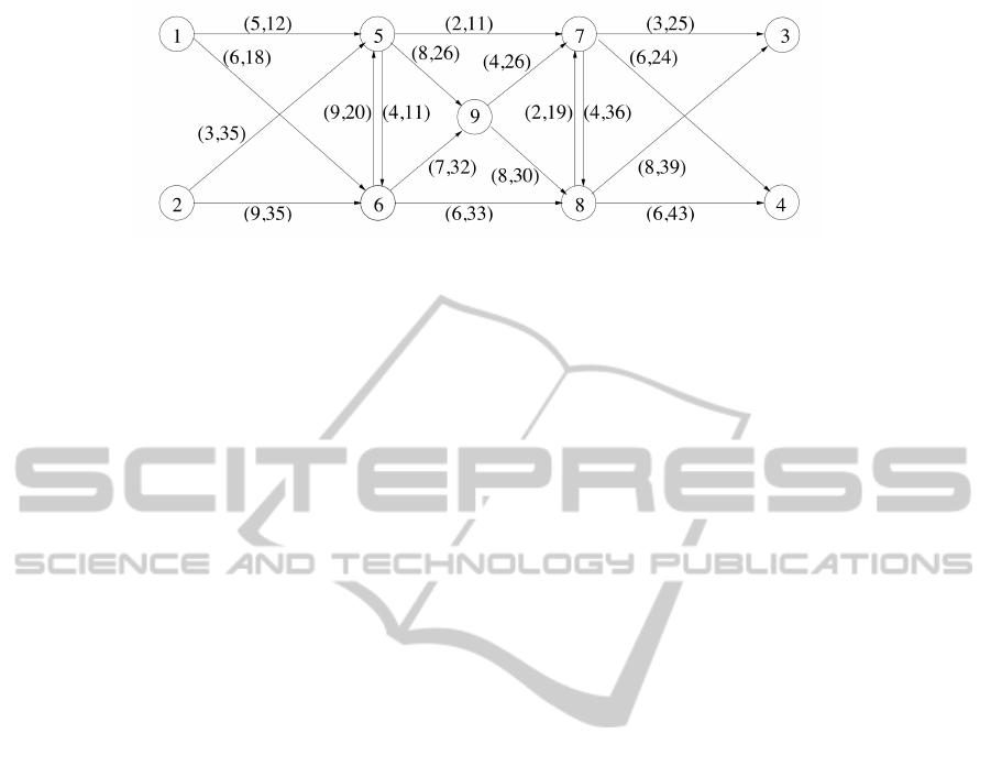
Figure 1: Nine Node Network.
4 NUMERICAL RESULTS
In this section, we present results obtained on a
benchmark network. In (Hearn and Ramana, 1998),
the authors propose different secondary objectives for
a toll problem. The problem MINSYS consists in
minimizing the total amount of toll.
In this section, we provide a comparison of our
multicommodity MINSYS algorithm, or MMINSYS,
introduced in this article, with the MINSYS algo-
rithm, on a synthetic network. We present results
for the Nine Node network described in (Hearn and
Ramana, 1998), and illustrated in figure 1. The arcs
are given “Bureau of Public Roads” (BPR) latency
functions. The tuple near an arc denotes its free flow
travel time followed by its capacity in the sense of
BPR. There are four OD pairs, with four different
travel demands.
OD pair: [1,3] [1,4] [2,3] [2,4]
Demand: 10 20 30 40
Results are presented in table 1. The aggregate
flow and commodity flows corresponding to the dif-
ferent OD pairs, at social optimum, are explicited for
each arc of the network. Origin based-arc tolls, solu-
tion of the algorithm 2, are also listed.
The Λ
k
, potential difference between the desti-
nation and the origin, are respectively 30.59, 29.21,
32.95, 31.57 for the above OD pairs. It is also an
upper bound to the tolls charged to one user of the
OD pair. As journeys for the different OD pairs are
similar in terms of travel times, the fixed part (which
does not depend on the path choosen by the user) is
approximately the same for each commodity.
A comparison of general properties of MMINSYS
program with other secondary objectives is presented
in table 2. The toll vectors are computed as explained
in the previous section.
Let us focus on the new formulation MMINSYS
compared to the other classical programs.
• MMINSYS solution gives a lower total of tolls
than MINSYS. This is mathematically evident, as
MINSYS is a problem restriction of MMINSYS.
MMINSYS total tolls are 9.5 % lower: allowing
multicommodity tolls helps minimizing the total
number of tolls raised.
• MMINSYS solution gives also interesting values
for the number of tolled arcs or for the maxi-
mum arc toll: there are respectively 4 and 5 arcs
tolled for origins 0 and 1, which represents 5 arcs
tolled to the operator point of view. The maxi-
mum arc toll is 8.00 for one commodity, 12.00 for
the other, which is greater than MINSYS solution
and MINTB solution (identical in this problem).
• The main benefit of this new algorithm is that the
pricing vector has an analytical expression and
can be computed in a linear time in the product of
the number of arcs of the network and the number
of different origins of the OD pairs. It does not
need numerical solvers. On the contrary, MIN-
SYS is the solution of a linear program with poly-
nomial complexity, not expected to be linear in
general.
5 CONCLUSIONS
In this article, we introduce the notion of commodity-
based potential pricing in order to design optimal
OD-pair differentiated congestion charges, in the con-
text of real-time GPS sensing. Our contributions in-
clude the mathematical construction and analysis of
commodity-based potential pricing schemes, the de-
sign of algorithmic methods for efficient computation
of these potentials, and the theoretical and numerical
analysis of their properties.
We show that our potential-based formulation pro-
vides a new characterization of the set of pricing
schemes such that the charge incurred on each arc is
positive, whose existence is equivalent to the acyclic
property of the commodity flows. The proof of this
equivalence result is constructive, and is based on a
ICORES2013-InternationalConferenceonOperationsResearchandEnterpriseSystems
148

Table 1: Nine Node Network - Flows and tolls for each commodity (tolls are identical for OD pairs with same origin).
Arc From to Aggr. flow Travel time Pair [1 3] Pair [1 4] Tolls Pair [2 3] Pair [2 4] Tolls
0 1 5 9.411 5.283 3.976 5.435 0. 0.000 0.000 0.
1 1 6 20.589 7.540 6.024 14.565 0. 0.000 0.000 0.
2 2 5 38.334 3.648 0.000 0.000 0. 22.185 16.149 0.
3 2 6 31.666 9.905 0.000 0.000 0. 7.815 23.851 0.
4 5 6 0.000 9.000 0.000 0.000 0. 0.000 0.000 0.
5 5 7 21.303 6.220 2.104 3.029 8. 7.569 8.602 12.
6 5 9 26.442 9.283 1.872 2.406 0. 14.617 7.547 4.
7 6 5 0.000 4.000 0.000 0.000 0. 0.000 0.000 0.
8 6 8 39.474 7.843 2.361 11.145 7.2 4.501 21.467 7.2
9 6 9 12.781 7.027 3.664 3.420 0. 3.313 2.384 0.
10 7 3 29.608 3.885 6.042 0.000 7.2 23.566 0.000 7.2
11 7 4 20.757 6.503 0.000 6.390 3.2 0.000 14.367 3.2
12 7 8 0.000 2.000 0.000 0.000 0. 0.000 0.000 0.
13 8 3 10.392 8.007 3.958 0.000 0. 6.434 0.000 0.
14 8 4 39.243 6.625 0.000 13.610 0. 0.000 25.633 0.
15 8 7 0.000 4.000 0.000 0.000 0. 0.000 0.000 0.
16 9 7 29.062 4.937 3.938 3.361 0. 15.997 5.765 0.
17 9 8 10.162 8.015 1.597 2.465 0. 1.933 4.166 0.
Table 2: Nine Node Network - Alternative Tolls.
SO total time 2253.92
UE total time 2455.84 (8.95% greater)
Problem solution MSCP MINSYS MINMAX MINTB MMINSYS
Total tolls 1493.46 887.57 1167.57 887.57 803.6
Total tolls / SO total time (%) 66.38 39.38 51.80 66.38 35.65
Number of toll booths 14 5 7 5 6
Max. arc toll 16.88 11.20 8.00 11.20 12.00
linear algorithm for the definition of a minimal posi-
tive pricing scheme.
Further directions of research include applications
of this new formulation to efficient computation of
more complex constrained network pricing problems:
robustness of pricing schemes around the social op-
timum, introduction of multi-class users or more so-
phisticated modeling of users preferences.
REFERENCES
Beckmann, M., McGuire, C. B., and Winsten, C. B. (1956).
Studies in the Economics of Transportation. Yale Uni-
versity Press.
Boyd, S. and Vandenberghe, L. (2004). Convex Optimiza-
tion. Cambridge University Press.
Braess, D. (1968).
¨
Uber ein paradoxon aus der verkehrspla-
nung. Unternehmensforschung, 12.
Dafermos, S. (1980). Traffic equilibrium and variational
inequalities. Transportation Science, pages 42–54.
Dahl, J. and Vandenberghe, L. (2008). Cvxopt: A python
package for convex optimization.
Hearn, D. W. and Ramana, M. V. (1998). Solving conges-
tion toll pricing models. Equilibrium and Advanced
Transportation Modeling, pages 109–124.
Mobile Millenium (2008). http://traffic.berkeley.edu.
Papadimitriou, C. (2001). Algorithms, games, and the in-
ternet. In Proceedings of the 33rd Annual ACM Sym-
posium on the Theory of Computing, pages 749 – 753.
Pigou, A. (1920). Wealth and Welfare. Macmillan, London.
Vickrey, W. (1969). Congestion theory and transport invest-
ment. The American Economic Review, 59:251–260.
LagrangianRoadPricing
149