
Dynamic 3D Mapping
Visual Estimation of Independent Motions for 3D Structures in Dynamic
Environments
Juan Carlos Ramirez and Darius Burschka
Faculty for Informatics, Technische Universitaet Muenchen, Boltzmannstrasse 3, Garching bei Muenchen, Germany
Keywords:
3D Mapping, 3D Blobs, Octree, Blobtree, Data Fusion, Ransac, Visual Motion Estimation.
Abstract:
This paper describes an approach to consistently model and characterize potential object candidates presented
in non-static scenes. With a stereo camera rig we recollect and collate range data from different views around
a scene. Three principal procedures support our method: i) the segmentation of the captured range images
into 3D clusters or blobs, by which we obtain a first gross impression of the spatial structure of the scene, ii)
the maintenance and reliability of the map, which is obtained through the fusion of the captured and mapped
data to which we assign a degree of existence (confidence value), iii) the visual motion estimation of potential
object candidates, through the combination of the texture and 3D-spatial information, allows not only to update
the state of the actors and perceive their changes in a scene, but also to maintain and refine their individual
3D structures over time. The validation of the visual motion estimation is supported by a dual-layered 3D-
mapping framework in which we are able to store the geometric and abstract properties of the mapped entities
or blobs, and determine which entities were moved in order to update the map to the actual scene state.
1 INTRODUCTION
Nowadays, besides the challenging task of building a
reliable 2- or 3D map, the principal objective in many
robot applications is to interact with the immediate
environment. For this, the robot system must be able
to correctly identify the objects or actors along with
their functions inside a scene in order to plan the ap-
propriated strategies of interaction. The challenge in-
creases in non-static environments in which the regis-
tration of 3D data (in a geometric level) and identifi-
cation of the actors (in an abstract level) become more
complex tasks. The system is then demanded to cope
not only with the imprecision and inherent noise of
the sensory data but also with the dynamic changes of
the scene, and a constant update to the current state re-
quires also a constant and consistent refinement of the
mapped information with the newly captured state. In
this context, an important mechanism for the percep-
tion of and update to new states is that of the estima-
tion of both independent- and ego-motion parameters
of the actors and camera rig for a correct estimation
of the expectations, see Fig. 1. Unlike works related
to structure from motion (SfM) in which mostly the
flow of salient information is detected, through the
combination of texture and spatial information we are
Figure 1: Overview of the approach. (Left) Image of the
scene at the first camera pose, (middle) tentative object
candidates, or 3D blobs, are identified after scene segmen-
tation, (right) independent- and ego-motion are estimated
from the first to the second pose.
also able to preserve and refine at the same time the
moving 3D structures. Our approach utilizes exclu-
sively visual information and discriminates between
the data that support the ego-motion (inliers) and that
caused by independent-object motions (outliers) un-
der a ransac scoring scheme. Having a set of matched
features either in 2- or 3D of a scene observed from
two different poses at different times, we profit from
the fact that not all the information classified as outlier
is derived from noisy or mismatched data, and this in-
formation gives, in turn, patterns indicating probable
independent events inside the same scene. In order
to detect these good outliers we utilize a dual-layered
framework that stores the elements as 3D blobs repre-
senting tentative object candidates; The advantage of
402
Ramirez J. and Burschka D..
Dynamic 3D Mapping - Visual Estimation of Independent Motions for 3D Structures in Dynamic Environments.
DOI: 10.5220/0004288004020406
In Proceedings of the International Conference on Computer Vision Theory and Applications (VISAPP-2013), pages 402-406
ISBN: 978-989-8565-48-8
Copyright
c
2013 SCITEPRESS (Science and Technology Publications, Lda.)

using this framework is twofold: i) in this work, the
geometric layer of the framework helps to spatially
relate the mapped elements and the outlier positions,
ii) for future works, once a mapped element was de-
tected it was moved, additional properties like grasp-
ing points or labels like movable, unmovable, etc., can
be assigned to that element and stored in the abstract
layer of the framework.
Related Work. Works on motion estimation are
mainly related to the simultaneous localization and
mapping (SLAM) problem and visual odometry (VO)
methods; SLAM-based systems capture salient fea-
tures of the surroundings, build a rigid 2- or 3D
map out of them and improve with each observa-
tion the state of the map, i.e., the position of the
captured features and sensor devices. In the classic
SLAM, the environment is considered to be static,
and moving features are considered sources of noise
(e.g., (Kitt et al., 2010)). In (Lin and Wang, 2010)
and (Wang et al., 2003) present examples of aug-
mented approaches of SLAM adapted for dynamic
environments that take into account these non-static
elements: the objects (sparse features) that are not
consistent regarding the robot motion are simply dis-
carded for being mapped and for the ego-motion esti-
mation, but they are tracked instead. In (Nister et al.,
2004) is presented a VO system for single and stereo
camera; it describes the basic steps like feature detec-
tion, feature matching and the robust pose estimation
which also employs a ransac scheme. One of the prin-
cipal steps, however, for any augmented version of
VO or SLAM is how to distinguish between the static
and non-static features. In (Lin and Wang, 2010) two
’SLAMs’ are initialized per new extracted feature, one
with and the other without adding such feature. After
that, they define a chi-square distance indicating the
difference of these two SLAM hypotheses; this dis-
tance is integrated using a binary Bayes filter whose
output is compared with a predetermined threshold;
after a fixed number of updates the feature is classified
as static or moving. In (Wang et al., 2011) they use
a single camera; the moving-object detection mecha-
nism is based on the correspondence constraint of the
essential matrix which is calculated using an extended
Kalman filter (EKF). For the moving-object tracking,
they used an EKF-based interacting multiple model
estimator (see references therein). A similar approach
to ours, coping with range data is described in (Moos-
mann and Fraichard, 2010).
The paper is organized as follows. Next section
describes briefly the 3D-mapping framework, in the
Sec. 3 we explain the visual motion estimation ap-
proach. The validation of the method is addressed in
Sec. 4 and in Sec. 5 some final comments and remarks
are made.
2 3D-MAPPING FRAMEWORK
The framework our approach is based on is described
in detail in (Ramirez and Burschka, 2011). In this sec-
tion we briefly present the two auxiliary procedures
supporting our approach: 3D segmentation and map
maintenance.
3D-Blob Detection. After the supporting-plane de-
tection, the rigid 3D reading is stored in an octree,
Fig. 2. In order to find the spatial relations among the
3D points a Depth-First Search (DFS) is performed
by traversing the leaves inside the octree and finally
identifying and clustering the connected components
as shown in Fig. 2.
Map Maintenance. This is done by validating or in-
validating the existence of each mapped point. For
this, a degree of existence or confidence value is as-
signed to each point during the blob fusion process:
every time a 3D point is fused its confidence value
is increased, otherwise its value is decreased. For
a proper confidence-value assignment, visibility tests
on each point are performed through a z-buffered re-
projection method.
Figure 2: Segmentation of a rigid 3D registration. (Left)
the range observation is stored in an octree, (right) segmen-
tation of the scene and clustering of the object candidates
are performed.
3 VISUAL MOTION ESTIMATION
At time k a set of N 3D points S(k) = {p
n
, P
n
} is
taken from the sensor devices, being p
n
∈ ℜ
3
the
measured, mean point value and P
n
its spatial un-
certainty matrix. After segmentation of S(k), we
define our map M(k) = {B
i
(k)} as a set of blobs
B
i
(k) = {p
j
, P
j
, γ
j
}, where each blob is composed by
a group of 3D points p
j
, with covariance matrix P
j
and an assigned confidence value γ
j
; we also main-
tain a set of 2D features I(k) = {u
f
, v
f
}, see Fig. 3,
with each of these pixel coordinate pairs having a cor-
responding 3D feature point in the set f(k) = (p
f
, P
f
)
Dynamic3DMapping-VisualEstimationofIndependentMotionsfor3DStructuresinDynamicEnvironments
403
related by H : (u
f
, v
f
) 7→ (p
f
, P
f
), where H is a map-
ping (3D stereo reconstruction) function of a feature
point from pixel to 3D coordinates. At pose (k + 1)
new sets {B
j
(k + 1)} and f(k + 1), from S(k + 1) and
I(k + 1), are determined and a set of L 2D-feature
correspondences C
2D
= (I
1
, I
2
) is established, where
I
1
⊆ I(k) and I
2
⊆ I(k + 1). The corresponding set of
3D matching points C
3D
= (F
1
, F
2
) is also determined
from C
2D
.
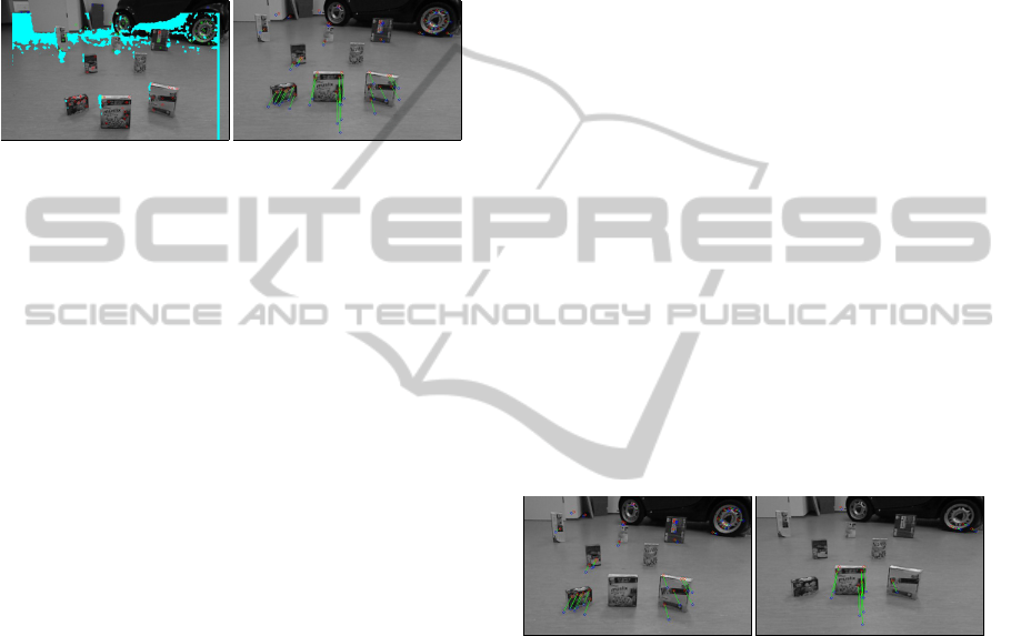
(a) (b)
Figure 3: Exemplary scene. The box closest to the camera
in (a) is moved back, while the cameras are moved forwards
(b). (a) First set of detected 2D features I(k) (the cyan-
shadowed areas do not contain depth information. (b) Flow
of valid 2D-feature matches C
2D
= (I
1
I
2
).
Ego-Motion Estimation. With these matching sets
we have defined a flow of visual features in 2- and
3D. In case of a static scene, all these lines converge
in one single point, the epipole, which is the projec-
tion of the previous camera-center pose in the current
camera screen and would correspond only to the mo-
tion of the cameras; the transformation that relates the
current pose with the previous one is then supported
ideally by all the matched feature points. In this case
we can find a rotation matrix
ego
R and a translation
vector
ego
t that minimize a cost function as proposed
in (Arun et al., 1987):
Σ
2
=
L
∑
l=1
kp
2,l
− (
ego
R · p
1,l
+
ego
t)k (1)
with p
1,l
∈ f
1,l
and p
2,l
∈ f
2,l
. Due to mainly noisy
sensor readings, feature mismatches and dynamic
changes in the environment, not all of the matched
features in {C
3D
} support the minimization in Eq. 1.
Therefore, we have to find a proper subset of matched
features (F
0
1
, F
0
2
) that is geometrically consistent with
the motion of the cameras. Under a ransac scor-
ing scheme we define the transformation hypothesis
(
hyp
R,
hyp
t), with the largest amount of scores, as the
one which gives this set of inliers. The scoring is
based on the similarity of the matching points:
p
0
1, j
=
hyp
R · p
1, j
+
hyp
t (2)
v
j j
= p
2, j
− p
0
1, j
(3)
χ
2
j
= v
j j
S
−1
j
v
T
j j
< χ
2
α
(4)
and
S
j
= P
1, j
+ P
2, j
(5)
where (p
1,l
, P
1,l
) ∈ F
1
and (p
2,l
, P
2,l
) ∈ F
2
. We use
the set of matched points that fulfill the Mahalanobis
metric χ
2
of Eq. 4 to minimize the sum of squared
residuals Σ
2
of Eq. 1 and to obtain the transformation
from pose k to pose (k + 1) corresponding to the
ego-motion of the cameras. The matched pairs
that do not fulfill Eq. 4 constitute the group of out-
liers. In Fig. 4(left) only the set of inliers is displayed.
Object-Motion Estimation. Outliers can be gener-
ated basically by three types of sources: noisy read-
ings, mismatched features and independent flows of
features. In order to detect each independent object
motion we determine the spatial relations that these
tracks give between the mapped and newly captured
blobs. Detecting that some outliers in F
1
and their
correspondences in F
2
belong to some blobs at time
k and (k + 1) respectively, i.e., {( f
1,l
)
i
} ∈ B
m
(k) and
{( f
2,l
)
i
} ∈ B
n
(k + 1), we infer that blob B
m
(k) was
moved to blob B
n
(k + 1) and compute its motion pa-
rameters (
n
R,
n
t) by following the same procedure for
the ego-motion estimation but now with a reduced set
of I outliers {( f
1,l
), ( f
2,l
)}
i
7→ (
n
R,
n
t). Fig. 4(right)
shows the subset of outliers from the set of matches
shown in Fig. 3(b).
Figure 4: Subsets of inliers indicating the ego-motion (left),
and outliers indicating the motion of the box (right).
4 EXPERIMENTS AND RESULTS
Our vision system is mounted on a wheeled robot that
moves to fixed poses observing a scene. The distances
and turning angles between any two positions are not
so big in order to obtain overlapped regions of cap-
tured data. The scene is constituted by some mov-
able, graspable objects, Fig. 5, that were moved as
the robot moved from one spot to the next. In order
to have a ground truth some marks were drawn on the
floor indicating at each step the new actual poses of
the objects and the robot; the marks are not percepti-
ble to the cameras. The robot was manually operated
in order to achieve the desired pose on the floor as
close as possible. Table 1 enumerates the sequence of
VISAPP2013-InternationalConferenceonComputerVisionTheoryandApplications
404
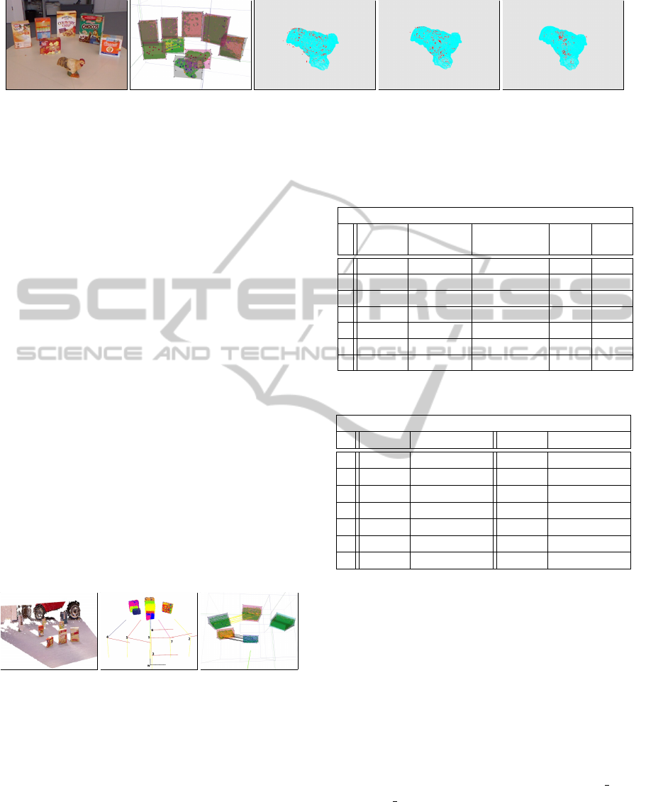
(a) (b) (c) (d) (e)
Figure 6: A series of range images of a complex object was collated. (a) A scene image from the sequence, (b) the 3D blob
map recognizes that two objects were moved, their states will be updated, (c-e) ICP fitting of blob valuated points with the
3D object model, see Table 3.
poses, the set-point values at each spot and the esti-
mated poses corresponding to a single trial. Consid-
ering that in this experiment the camera positions are
biased by a human factor regarding the manual op-
eration of the robot, in Table 1 we also report as a
reference, the pose values that were obtained by mov-
ing the robot and keeping the same scene static. Con-
cerning the dynamic scene, since the estimation of a
transformation depends on the quantity as well as the
quality of the points, we also include in the table the
mean squared error (MSE) of each transformation as
a measured of the reliability or precision of the esti-
mation (MSE Tr), and in order to have a statistics of
the accuracy of the process, we show the MSE of the
Euclidean distance (MSE Eu) between the estimated
poses and the reference positions corresponding to 40
measurements in each pose. Because we aim at build-
ing a 3D map for robot interaction, only the objects
that lie closer to the stereo rig, inside a radius of 2m
from the cameras, are registered into the map, in our
example this corresponds to the first three boxes in
Fig. 5(a). This figure shows a textured 3D image at
the first state of the scene. Fig. 5(b) shows by color all
the static registrations along with the estimated cam-
era pose frames for each step of the sequence. The
(a) (b) (c)
Figure 5: Visual motion estimations. (a) Textured 3D image
of the scene at its initial state, (b) robot-pose frames and
static registrations, (c) detection of motion in two mapped
objects.
last two columns of Table 1 indicate that our motion
estimation system is more precise than accurate, i.e.,
we can not certainly determine the absolute pose of
each mapped object in the world but rather determine
that the geometric relations in the map measured ei-
ther between any two of them or locally to a single
blob are the closest values to the actual ones. In Ta-
Table 1: Results of the ego-motion estimation.
Pose (X[cm], Y[cm], angle[
◦
])
Set Static Dynamic MSE MSE
Point Scene Scene Tr(x
−3
) Eu
1
(0,0,0) (0,0,0) (0,0,0) —– —-
2
(40,0,10) (41.21,-0,9.7) (42.25,0,10.46) 1.019 6.9104
3
(0,-20,0) (-0,-19.54,0.88) (0,-20.12,0.15) 1.029 1.5678
4
(-45,0,15) (-46.19,-0,14.71) (-45.16,-0,14.0) 0.119 3.3030
5
(-24,0,14) (-23.62,-0,14,32) (-24.72,-2,13.78) 0.282 5.9464
6
(0,10,0) (-0,9.65.4,1.1) (1.1,8.32,0.44) 0.688 3.6485
7
(20,0,10) (20,0,9.7) (22.22,-0,11.35) 0.316 5.8045
Table 2: Results of the object-motion estimation.
Pose (X[cm], Y[cm], angle[
◦
])
Set Point Cereal Box Set Point Pop Corn Box
1
(0,120,0) (0,117,1.52) (-33,115,10) (-33.67,114,8.1)
2
(0,110,0) (0,106.3,0.28) (-33,115,10) (33.84,113.42,9.52)
3
(0,130,0) (0,126.3,1.92) (-33,115,10) (33.78,113.01,8.78)
4
(0,130,0) (0,126.52,2.39) (-27,107,10) (-27.42,104.95,7.40)
5
(-33,120,10) (-32.77,118.28,4.81) (0,100,0) (0,97.15,1.16)
6
(-33,120,10) (-32.74,118.27,5.46) (0,94,0) (1.38,92.84,1.24)
7
(-33,120,10) (-32.83,118.22,6.04) (0,94,20) (0,92.42,22.47)
ble 2 we report the estimated pose values that were
obtained with the moved objects. We now present the
results of collating a sequence of range data of a non-
simple geometric model in Fig. 6(a). The object and
the cameras were moved to different spots during the
sequence. In order to show how precise the different
sets of valuated points of a 3D-blob image the actual
mapped object, we present the results of fitting by ICP
each point set to a 3D model of the mapped object.The
confidence value assignments ranges from 0-7. Some
fittings can be visually observed in Fig. 6(c-e). We
also present the magnitude of the matrix rotation,
Eq. 6, that was needed for each fitting: {valuated pts}
→ {model pts}. Since the object-model frame and
the valuated-point frame were aligned before running
ICP, this value will give us a measure of the amount
of correction that was needed to obtain a correspond-
ing RMS error value of this fitting. The results are
shown in Table 3. Although the amount of correction
Dynamic3DMapping-VisualEstimationofIndependentMotionsfor3DStructuresinDynamicEnvironments
405

Table 3: Results of the confidence value γ assignments.
Chicken Object Blob
γ
Points Rotation RMS
Figure
[%] Norm Error
7 1.97 0.257931 0.001407 Fig. 6(e)
6 2.85 0.279540 0.001439 Fig. 6(d)
5 3.24 0.334356 0.002410 Fig. 6(c)
4 74.66 0.411679 0.004266 —–
3 4.92 0.339462 0.004003 —–
2 4.14 0.255960 0.002779 —–
1 3.01 0.260456 0.002608 —–
0 5.22 0.251197 0.002689 —–
is similar for the points with extreme confidence val-
ues, we can observe that the points with larger confi-
dence values present smaller RMS errors; this means
that these points were better spatially located in their
local frame before the ICP fitting and therefore de-
scribe better the actual size of the object.
kR
F
k ≡ k{valuated pts} − {model pts}k
F
=
q
trace(R
T
· R) (6)
5 CONCLUSIONS
In this work we presented a feature-based updating
mechanism for 3D structures. This mechanism along
with ransac are the basis for our independent-motion
estimation method in which we exploit the informa-
tion the outliers can convey under the assumption that
not all of them are produced by noisy readings or mis-
matched features. While the inliers describe the ego-
motion, with the set of good outliers we are able to
infer the rest of independent motion parameters. For
detection of this latter set we utilize the geometric
layer of presented mapping framework. The experi-
ments carried out utilized exclusively visual informa-
tion and yielded precise results regarding the pose es-
timation between two consecutive spots. In the other
hand, since our approach is based on ransac some
drawbacks are also inherited from it: the ego-motion
estimation relies on the detection of the set of inliers
which in ransac is composed by the majority of the
captured elements. In highly dynamic environments,
however, the ego-motion estimation might not be sup-
ported by most of the measured elements; in such a
case other additional mechanisms like wheel-encoder
based odometry, global position system (GPS), iner-
tial measurement unit (IMU), etc. can be integrated.
ACKNOWLEDGEMENTS
This work was supported by the DAAD-Conacyt In-
terchange Program A/06/13408 and partially sup-
ported by the European Community Seventh Frame-
work Programme FP7/2007-2013 under grant agree-
ment 215821 (GRASP project).
REFERENCES
Arun, K. S., Huang, T. S., and Blostein, S. D. (1987). Least-
squares fitting of two 3-d point sets. IEEE Trans. Pat-
tern Anal. Mach. Intell., 9(5):698–700.
Kitt, B., Geiger, A., and Lategahn, H. (2010). Visual odom-
etry based on stereo image sequences with ransac-
based outlier rejection scheme. In Intelligent Vehicles
Symposium (IV), 2010 IEEE, pages 486 –492.
Lin, K.-H. and Wang, C.-C. (2010). Stereo-based simulta-
neous localization, mapping and moving object track-
ing. In Intelligent Robots and Systems (IROS), 2010
IEEE/RSJ International Conference on, pages 3975 –
3980.
Moosmann, F. and Fraichard, T. (2010). Motion estima-
tion from range images in dynamic outdoor scenes. In
Robotics and Automation (ICRA), 2010 IEEE Interna-
tional Conference on, pages 142 –147.
Nister, D., Naroditsky, O., and Bergen, J. (2004). Visual
odometry. In Computer Vision and Pattern Recogni-
tion, 2004. CVPR 2004. Proceedings of the 2004 IEEE
Computer Society Conference on, volume 1, pages I–
652 – I–659 Vol.1.
Ramirez, J. and Burschka, D. (2011). Framework for con-
sistent maintenance of geometric data and abstract
task-knowledge from range observations. In Robotics
and Biomimetics (ROBIO), 2011 IEEE International
Conference on. To be published.
Wang, C.-C., Thorpe, C., and Thrun, S. (2003). Online si-
multaneous localization and mapping with detection
and tracking of moving objects: theory and results
from a ground vehicle in crowded urban areas. In
Robotics and Automation, 2003. Proceedings. ICRA
’03. IEEE International Conference on, volume 1,
pages 842 – 849 vol.1.
Wang, Y.-T., Feng, Y.-C., and Hung, D.-Y. (2011). De-
tection and tracking of moving objects in slam using
vision sensors. In Instrumentation and Measurement
Technology Conference (I2MTC), 2011 IEEE, pages 1
–5.
VISAPP2013-InternationalConferenceonComputerVisionTheoryandApplications
406
