FlexRender: A Distributed Rendering Architecture for Ray Tracing

Huge Scenes on Commodity Hardware

Bob Somers and Zo

e J. Wood

California Polytechnic University, San Luis Obispo, CA, U.S.A.

Keywords:

Rendering, Distributed Rendering, Cluster Computing.

Abstract:

As the quest for more realistic computer graphics marches steadily on, the demand for rich and detailed im-

agery is greater than ever. However, the current “sweet spot” in terms of price, power consumption, and perfor-

mance is in commodity hardware. If we desire to render scenes with tens or hundreds of millions of polygons

as cheaply as possible, we need a way of doing so that maximizes the use of the commodity hardware that we

already have at our disposal. We propose a distributed rendering architecture based on message-passing that

is designed to partition scene geometry across a cluster of commodity machines, allowing the entire scene to

remain in-core and enabling parallel construction of hierarchical spatial acceleration structures. The design

uses feed-forward, asynchronous messages to allow distributed traversal of acceleration structures and evalu-

ation of shaders without maintaining any suspended shader execution state. We also provide a simple method

for throttling work generation to keep message queueing overhead small. The results of our implementation

show roughly an order of magnitude speedup in rendering time compared to image plane decomposition, while

keeping memory overhead for message queuing around 1%.

1 INTRODUCTION

Rendering has advanced at an incredible pace in re-

cent years. At the heart of rendering is describing the

world we wish to draw, which has traditionally been

done by deﬁning surfaces. While exciting develop-

ments in volume rendering techniques happen on a

regular basis, it is unlikely we will abandon surface

rendering any time soon. The champion of surface

representations in rendering, has been the polygonal

mesh. Even when used to store smooth surfaces in a

compressed way (as with subdivision surfaces), they

are usually tesselated into large numbers of ﬁne poly-

gons for rendering. Since their representation is de-

ﬁned explicitly, meshes with ﬁne levels of detail have

signiﬁcantly higher storage requirements. Thus, as

the demand for higher visual ﬁdelity increases, the

natural tendency is to increase geometric complexity.

Graphics, and ray tracing in particular, has long

been said to be a problem that is embarrassingly par-

allel, given that many graphics algorithms operate

on pixels independently. Graphics processing units

(GPUs) have exploited this fact for years to achieve

amazing throughput of graphics primitives in real-

time. While processor architectures have become ex-

ceedingly parallel and posted impressive speedups,

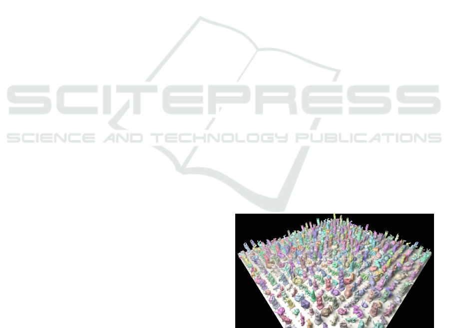
Figure 1: Field of high resolution meshes whose geometric

complexity is nearly 87 million triangles. Rendered across

4 commodity machines using FlexRender.

the memory hierarchy has not had time to catch up.

For a processor to perform well, the CPI, cycles per

instruction, must remain low to ensure time is spent

doing useful work and not waiting on data.

In current memory hierarchies, data access time

can take anywhere from around 12 cycles (4 nanosec-

onds for an L1 cache hit) to over 300 cycles (100

nanoseconds for main memory). Techniques such

as out-of-order execution are helpful in ﬁlling this

wasted time, but for memory intensive applications

it can be difﬁcult to ﬁll all the gaps with useful work.

Because of this fact, there is a lot more to paral-

152

Somers B. and J. Wood Z..

FlexRender: A Distributed Rendering Architecture for Ray Tracing Huge Scenes on Commodity Hardware.

DOI: 10.5220/0004289501520164

In Proceedings of the International Conference on Computer Graphics Theory and Applications and International Conference on Information

Visualization Theory and Applications (GRAPP-2013), pages 152-164

ISBN: 978-989-8565-46-4

 2013 SCITEPRESS (Science and Technology Publications, Lda.)

lel rendering than initially meets the eye. Graphics

may indeed by highly parallel, but its voracious ap-

petite for memory access is actively working against

its parallel efﬁciency on current architectures.

This paper presents FlexRender, a ray tracer de-

signed for rendering scenes with high geometric com-

plexity on commodity hardware. We speciﬁcally tar-

get commodity hardware because it currently has an

excellent cost to performance ratio, but still typically

lacks enough memory to ﬁt large scenes entirely in

RAM.

Our work describes the following core contribu-

tions:

1. A feed-forward messaging design between work-

ers that passes enough state with every ray to

never require reply messages.

2. An approach to shading using this messaging de-

sign that does not require suspending execution of

shaders and maintaining suspended state.

3. An extension to a stackless BVH traversal algo-

rithm (Hapala et al., 2011) that makes it possible

to suspend traversal at one worker and resume it

at another.

4. A simple throttling method for managing memory

overhead for message queueing without resorting

to a complicated dynamic scheduling algorithm.

5. Technical insight into the challenges of building

such a renderer, an analysis of our results, and an

open-source implementation.

In particular, we show that FlexRender can

achieve speedups that are around an order of magni-

tude better than image plane decomposition for com-

modity machines, and can naturally self-regulate the

cluster of workers to keep the memory overhead due

to message queuing around 1% of each worker’s main

memory.

It is important to remember that FlexRender is

an experimental design, and some of our design

goals worked better than others. In the hopes of

making future experimentation easier for others, we

provide the complete source code of FlexRender at

http://www.ﬂexrender.org.

2 BACKGROUND

FlexRender leverages observations from several fun-

damental building blocks, including Radiometry,

bounding volume hierarchies, and Morton coding.

Radiometry. For the purposes of FlexRender, we

note the following observations of the radiometry

model of light:

Light Behaves Linearly. The combined effect of

two rays of light in a scene is the same as the sum

of their independent effects on the scene.

Energy is Conserved. When a ray reﬂects off of a

surface, it can never do so with more energy than

it started with.

FlexRender exploits these observations in the follow-

ing ways:

The Location of Computation does not Matter. If

the scene is distributed across many machines, it

makes no difference which machine computes the

effect of a ray. The sum of all computations will

be the same as if all the work was performed on a

single machine.

Transmittance Models Energy Conservation. If

we store the amount of energy traveling along

a ray (the transmittance) with the ray itself, we

need not know anything about the preceding

rays or state that brought this ray into existence.

We can compute its contribution to the scene

independently and ensure that linearity and

energy conservation are both respected.

Bounding Volume Hierarchies. The traversal al-

gorithm of a BVH is naturally recursive, but recursive

implementations keep their state on the call stack. In

FlexRender, BVH traversal may need to be suspended

on one machine and resumed it on another, so all

of the traversal state needs to be explicitly exposed.

Refactoring it as an iterative traversal explicitly ex-

poses the state for capturing, but unfortunately it still

requires a traversal stack of child nodes that must be

visited on the way back up the tree. In FlexRender,

rays carry all necessary state along with them, and

this approach would require the entire stack to be in-

cluded as ray state.

However, (Hapala et al., 2011) presents a stack-

less traversal method. The key insight is that if parent

links are stored in the tree, the same traversal can be

achieved using a three-state automaton describing the

direction you came from when you reached the cur-

rent node (i.e. from the parent, from the sibling, or

from the child). They show that their traversal algo-

rithm produces identical tree walks and never retests

nodes that have already been tested.

FlexRender leverages this traversal algorithm due

to its low state storage requirements. Each ray only

needs to know the index of the current node it is

traversing and the state of the traversal automaton.

FlexRender:ADistributedRenderingArchitectureforRayTracingHugeScenesonCommodityHardware

153

Morton Coding and the Z-Order Curve. Morton

coding is a method for mapping coordinates in multi-

dimensional space to a single dimension. In particu-

lar, walking the multidimensional space with a Mor-

ton coding produces a space-ﬁlling Z-order curve.

Figure 2: Examples of two dimensional and three di-

mensional Z-order curves. Credit: “David Eppstein” and

“Robert Dickau” (Creative Commons License).

More concretely, FlexRender needs to distribute

scene data to machines in the cluster, without a pre-

processing step, in a spatially coherent way. If the ge-

ometry on each machine consists of a localized patch

of the overall geometry, it allows us to minimize com-

munication between the machines, and thus, only pay

the network cost when absolutely needed.

Because the Morton coding produces a spatially

coherent traversal of 3D space, dividing up the 1D

Morton code address space among all the machines

participating in the render gives a reasonable assur-

ance of spatial locality for the geometry sent to each

machine.

The Morton coding is also simple to implement.

For example, to map a point P in a region of 3D

space (deﬁned by its bounding extents min and max)

to a Morton-coded 64-bit integer, discretizing each

axis evenly allows for 21 bits per axis, yielding a 63-

bit address space (and one unused bit in the integer).

We compute the Morton code by calculating the 21-

bit discretized component of P along each axis, then

shifting the components from each axis into the 64-bit

integer one bit at a time from the most-signiﬁcant to

least-signiﬁcant bit.

3 RELATED WORK

A number of algorithms are designed to completely

avoid large amounts of geometry altogether. Dis-

placement maps (Krishnamurthy and Levoy, 1996)

and normal maps using texture data (Cohen et al.,

1998) and (Cignoni et al., 1998) are commonly used,

especially in real-time applications. However, normal

mapping displays visual artifacts, particularly around

the edges of the mesh or in areas where the tex-

ture is stretched or compressed. Similarly, level of

detail is commonly used to replace high resolution

meshes with lower resolution versions when they are

far enough away from the viewer (Clark, 1976). How-

ever, it requires the creation of multiple resolution

meshes and algorithms to smoothly handle resolution

changes.

More recently, (Djeu et al., 2011) provides a

framework for efﬁciently tracing multiresolution ge-

ometry, but it has large memory requirements and is

not applied to clusters of commodity machines. Sim-

ilarly (

Afra, 2012) presents a voxel-based paging sys-

tem designed for interactive use, but it requires an

expensive preprocessing step and displays visual ar-

tifacts at low LOD levels.

In (DeMarle et al., 2004), distributed shared mem-

ory is used to page in necessary data for rendering,

but it relies on a complicated task scheduler to avoid

ﬂooding the network with large data blocks and it

suffers from cache storms in a multithreaded envi-

ronment. Efﬁcient memory use is also the focus of

(Moon et al., 2010), which obtains an order of mag-

nitude speedup from reordering ray evaluation in a

cache-oblivious way. This approach would comple-

ment our method very well.

The focus of (Reinhard et al., 1999), was devel-

opment of a hybrid work scheduler which would im-

prove performance with more effective hardware uti-

lization, but it had problems with high memory over-

head. Earlier this year, (Navr

atil et al., 2012) pre-

sented an improved approach which uses a dynamic

scheduler to move work from an image plane decom-

position to a domain decomposition as rays begin to

diverge.

A similar approach to ours was presented in

(Badouel et al., 1994), but it failed to address the issue

of shader execution within their asynchronous clus-

ter design. Another similar approach is the Kilauea

renderer in (Kato and Saito, 2002), but its pipeline is

very latency sensitive and network communication is

heavy due to rays being duplicated across many work-

ers.

Recent research in strict out-of-core methods has

focused on techniques for using main memory as an

efﬁcient cache. In (Kontkanen et al., 2011), they

present a technique for dealing with huge point clouds

used in point-based global illumination and demon-

strate impressive cache hit rates of 95% and higher.

Prior to that, (Pantaleoni et al., 2010) generated di-

rectional occlusion data using ray tracing, which was

compressed into spherical harmonics for evaluation at

render time. Ray tracing was not used for primary vis-

ibility. Like FlexRender, they also used hierarchical

BVHs, but for the purpose of chunking scene data into

GRAPP2013-InternationalConferenceonComputerGraphicsTheoryandApplications

154

units of work that could be loaded into main memory

quickly.

Using GPGPU techniques, (Garanzha et al.,

2011), presented a method for ray tracing large scenes

that are out-of-core on the GPU. Parts of their archi-

tecture are similar to FlexRender on a single-device

scale, speciﬁcally their use of hierarchical BVHs and

ray queues to handle rays cast from shaders. How-

ever, the global ray queue is fairly memory intensive,

potentially storing up to 32 million rays.

Leveraging MapReduce (Dean and Ghemawat,

2004), an implementation of a ray tracer was pre-

sented by (Northam and Smits, 2011), but sending

large amounts of scene data to workers signiﬁcantly

slowed down processing. Their solution was to break

the scene into small chunks and resolve the inter-

section tests in the reduce step. Unfortunately, this

does a lot of unnecessary work, because many non-

winning intersections are computed that would have

been pruned in a typical BVH traversal.

4 FlexRender ARCHITECTURE

In general, rendering with FlexRender proceeds in the

following way:

1. Read in the scene data and deﬁne the maximum

bounding extents of the entire scene. As data is

read in, it is distributed to the workers using the

Morton coding.

2. Once the scene is distributed, workers build BVHs

in parallel for their respective local region of the

scene. When complete, they send their maximum

bounding extents to the renderer.

3. The renderer constructs a top-level BVH from

each of the workers’ bounds and sends this top-

level BVH to all the workers.

4. Workers create image buffers. All shading com-

puted on a worker is written to its own buffer.

5. Workers cast primary rays from the camera and

test for intersections.

• During intersection testing, rays may be for-

warded over the network to another worker if

they need to test geometry within the bounding

extents of that worker.

• Once the nearest intersection is found, illumi-

nation ray messages are created and sent to

workers that have lights. These workers send

light rays back towards the point of intersection

to test for occlusion.

• If the light rays reach the original intersection,

the point is illuminated and the worker com-

putes shading.

6. Once all rays have been accounted for, work-

ers send their image buffers back to the renderer,

which composites them together into a ﬁnal im-

age.

In the next few sections, we will examine each part

of this process in greater detail.

4.1 Workers and the Renderer

There are two potential roles a machine can play dur-

ing the rendering process.

Worker. These machines receive a region of the

scene and act as ray processors, ﬁnding intersec-

tions computing shading. They produce an image

that is a component of the ﬁnal render. There may

be an arbitrary number of workers participating.

Renderer. This machine distributes scene data to the

workers. Once rendering begins it monitors the

status of the workers and halts any potential run-

away situations (see Section 4.4.3). When the

renderer decides the process is complete, it re-

quests the image components from each worker

and merges them into the ﬁnal image. There is

only a single renderer in any given cluster.

The network architecture is client/server con-

nected in a star topology. Each worker exposes a

server which processes messages and holds client

connections open to every other worker for pass-

ing messages around the cluster. The renderer also

holds a client connection to every worker for sending

conﬁguration data, preparing the cluster for render-

ing (described in Section 4.3), and monitoring render

progress (described in Section 4.5).

The current implementation does not include any

provisions for fault tolerance. However, there is no ar-

chitectural restriction preventing such measures. For

topics involving the design of robust and resilient

clusters, we refer the reader to the distributed systems

literature.

The graphics machinery is fairly straightforward.

A scene consists of a collection of meshes, which are

stored as indexed face sets of vertices and faces. Each

mesh is a assigned a material, which consists of a

shader and potentially a set of bindings from textures

to names in the shader. A shader is a small program

that computes the lighting on the surface at a particu-

lar point.

FlexRender:ADistributedRenderingArchitectureforRayTracingHugeScenesonCommodityHardware

155

4.2 Fat Rays

The core message type in FlexRender is the fat ray.

They are so named because they carry additional state

information along with their geometric deﬁnition of

an origin and a direction. Their counterparts, slim

rays, consist of only the geometric components.

Speciﬁcally, a fat ray contains the following data,

which is detailed in the subsequent sections:

• The type of ray this is.

• The source pixel that this ray contributes to.

• The bounce count, or number of times this ray

has reﬂected off a surface (to prevent inﬁnite

loops).

• The origin and direction of the ray.

• The ray’s transmittance, (related to the amount

of its ﬁnal pixel contribution).

• The emission from a light source carried along the

ray, if any.

• The target intersection point of the ray, if any.

• The traversal state of the top-level BVH.

• The hit record, which contains the worker, mesh,

and t value of the nearest intersection.

• The current worker this ray should be forwarded

to over the network.

• The number of workers touched by the ray. (Not

used for rendering, only analysis.)

• A next pointer for locally queuing rays. (Obvi-

ously invalid over the network.)

In total, the size of a fat ray is 128 bytes.

4.3 Render Preparation

To begin rendering FlexRender ensures that all the

workers agree on basic rendering parameters, such

as the minimum and maximum extents of the scene,

which is used for driving Morton coding discretiza-

tion along each axis. Once this data has been synchro-

nized with all workers, each worker establishes client

connections with every other worker that remain open

for the duration of the render.

The renderer then divides up the 63-bit Morton

code address space evenly by the number of workers

participating and assigns ranges of the address space

(which translate into regions of 3D space) to each

worker. At this point the renderer begins reading in

scene data and takes the following actions with each

mesh:

1. Compute the centroid of the mesh by averaging its

vertices.

2. Compute the Morton code of the mesh centroid.

The range this falls in determines which worker

the mesh will be sent to.

3. Ensure that any asset dependencies (such as ma-

terials, shaders, and textures) for this mesh are

present on the designated worker.

4. Send the mesh data to the designated worker.

5. Delete the mesh data from renderer memory.

Although the current implementation reads scene

data in at the renderer and distributes it over the net-

work, there is no inherent reason why it needs to do

so. For example, if all workers have access to shared

network storage, the renderer could simply instruct

each worker to load a particular mesh itself, reducing

load time.

4.3.1 Parallel Construction of Bounding Volume

Hierarchies

Next, workers construct a BVH for each mesh

they have for accelerating spatial queries against the

meshes. While building each BVH, the worker tracks

bounding extents of each mesh. Workers then build a

root BVH for the entire region owned by the worker

with the mesh extents as its leaf nodes. When testing

for intersections locally, a worker ﬁrst tests against

this root BVH to determine candidate meshes, then

traverses each mesh’s individual BVH to compute ab-

solute intersections. After construction of this root

BVH, the root node’s bounding extents describe the

spatial extent of all geometry owned by the worker.

Once construction of all local BVHs is complete,

workers send their root bounding extents to the ren-

derer. The renderer then constructs a ﬁnal top-level

BVH with worker extents as its leaf nodes. This top-

level BVH is then distributed to all workers. This is

a quick and lightweight process, since the number of

nodes is only 2n − 1, where n is the number of work-

ers. This top-level BVH guides where rays are sent

over the network in Section 4.4.4.

4.4 Ray Processing

Workers are essentially multithreaded ray processors.

Their general work consists of processing rays by test-

ing for intersection, potentially forwarding rays to an-

other worker, or computing shading values if a ray

terminates.

To manage these various tasks when all the geom-

etry and lights may not be local to the worker, there

are three different types of rays:

GRAPP2013-InternationalConferenceonComputerGraphicsTheoryandApplications

156

• Intersection rays are very much like traditional

rays, which identify points in space that require

shading.

• Illumination ray messages are copies of inter-

section rays that have terminated. They are sent

to workers who have emissive geometry and as-

sist in the computation of shading.

• Light rays are Monte Carlo samples that con-

tribute direct illumination to a point being shaded.

Figure 3: The three different ray types and their interac-

tions.

The typical lifetime of these various rays is as follows:

1. An intersection ray is cast into the scene.

2. When that intersection ray terminates at a point in

space, it dies and spawns an illumination ray mes-

sage sent to each worker with emissive geometry.

3. When those illumination ray messages are deliv-

ered, they die and spawn light rays cast toward the

original intersection.

4. If they terminate at the original intersection, the

worker computes shading for it. When those light

rays terminate, they die.

A single intersection ray can spawn many addi-

tional rays and light rays are the most likely to ter-

minate without generating additional rays. These are

key factors for deciding ray processing order for the

cluster.

4.4.1 Illumination

In FlexRenderer there is no special “light” type, only

meshes that are emissive, which is a property set by

the assigned material. Emissive meshes are known to

inject light into the scene through their shader. During

scene loading, the renderer maintains a list of workers

that have been sent at least one emissive mesh and

sends the list to all workers before rendering begins.

Once intersection testing has identiﬁed a point

needing shading, FlexRender must determine the vis-

ibility of light sources from that point. In a traditional

ray tracer, shadow rays are cast from the point of in-

tersection to sample points on the surface of the light

to determine visibility. However, from the perspective

of the worker computing shading, it has no idea where

the lights in the scene are, or if there is any geometry

occluding the light, it just knows which workers have

emissive meshes.

To solve this problem, illumination ray messages

are used to request that emissive meshes instead test

for visibility from their perspective. In this way,

FlexRender traces an equivalent of shadow rays but

in the opposite direction, which we call light rays. In-

stead of originating at the intersection point and trav-

eling in the direction of the light, they originate at

the light and travel in the direction of the intersec-

tion point. Area lights are supported through Monte

Carlo integration by creating multiple light rays with

origins sampled across the surface of the light.

If a light ray returns to the original intersection

point after being traced through the cluster, which can

be determined via the information carried forward in

the fat rays, the renderer knows its path from the light

was unoccluded. The advantage of this method is that

it leverages the same method for tracing rays through

a distributed BVH that used for testing ray intersec-

tions.

In summary, illuminating an intersection is done

as follows:

1. On the worker where an intersection was found,

copy the ray data into an illumination ray message

with the target set to the point of intersection.

2. Send the illumination ray message to all emissive

workers.

3. When a worker receives an illumination ray mes-

sage, generate sample points across the surface of

all emissive meshes. Set these sample points as

the origins for new light rays.

4. Set the directions of all the light rays such that

they are oriented in the direction of the target.

5. Push each light ray into the ray queue and let the

cluster process them as usual.

4.4.2 Ray Queues

To manage the various types and numerous rays

present in the system, each worker has a ray queue,

with typical push and pop operations. Internally, this

is implemented as three separate queues, where rays

are separated by type. It also contains information

about the scene camera, for generating new primary

rays. When a new ray arrives at a worker, it is im-

mediately pushed into the queue according to its type

(intersection, illumination, or light).

FlexRender:ADistributedRenderingArchitectureforRayTracingHugeScenesonCommodityHardware

157

When the worker pops a ray from the queue, rays

are pulled from the internal queues in the following

order:

1. The light queue, since these are least likely to

generate new rays.

2. If the light queue is empty, the worker pops from

the illumination queue, since these will generate

a limited number of new rays.

3. If the illumination queue is empty, the worker

pops from the intersection queue, since these can

generate the most new rays.

4. If all of the internal queues are empty, the worker

uses the camera to cast a new primary ray into the

scene

Processing rays as a priority queue is essential

for managing the exponential explosion of work than

can occur if too many primary rays enter the system

at once. It also helps reduce memory required for

queuing because new work is not generated until the

worker has nothing else to work on.

4.4.3 Primary Ray Casting

To give the cluster the ability to regulate itself, each

worker in the cluster is responsible for casting a por-

tion of the primary rays in the scene. Consider the

case where a worker has not received any work re-

cently from other workers in the cluster for whatever

reason. By giving the worker control over primary ray

casting for a portion of the scene, we enable workers

to generate work when they have nothing to do.

However, in the case where a worker contains

mostly background geometry, it will infrequently re-

ceive work from others because its size in screen

space is small, yet it is in charge of casting primary

rays for a larger slice of the image. In this case the

worker may go on an unfettered spree of primary ray

casting, generating lots of work for others and little

for itself. To prevent this “runaway” case from over-

burdening the ray queues, workers report statistics

about their progress to the renderer occasionally (10

times per second in our implementation). If a worker

is getting signiﬁcantly further ahead of the others in

primary ray casting, the renderer temporarily disables

primary ray casting on that worker.

This is not ideal, since lightly loaded workers will

wait idle until they receive work to do, but it is sim-

ple to implement and works remarkably well in prac-

tice for mitigating the ray explosion and associated

memory required for message queueing. See (Rein-

hard et al., 1999) and (Navr

atil et al., 2012) for more

sophisticated approaches that use dynamic scheduling

to increase performance.

4.4.4 Distributed BVH Traversal

Distributed traversal of the scene BVH happens at two

levels. Recall that the top level BVH contains bound-

ing boxes for each worker and is present on all work-

ers. Below that, each worker contains a BVH consist-

ing of only the mesh data present on that worker.

When a ray is generated, traversal begins at the

root of the top level tree and proceeds as described by

(Hapala et al., 2011). When a leaf node intersection

occurs closer to the camera than the current closest

intersection, the traversal state is packed into the ray

and the ray is forwarded to the candidate worker. The

packed traversal state includes the index of the cur-

rent top-level node and the state of the traversal au-

tomaton (from the parent, from the sibling, or from

the child). The logic for top-level traversal is shown

in Algorithm 1.

Algorithm 1: Top-level BVH traversal.

while current node ! = root do

if ray intersects leaf node then

if leaf node t < ray t then

pack traversal state into ray;

send ray to leaf node worker;

end

When a ray is received over the network and un-

packed at the next worker, the traversal state is exam-

ined. If the traversal state points to the root of the top-

level tree, the scene traversal has completed and the

worker can shade the intersection if it was the worker

on which that intersection occurred. Otherwise, the

ray must be forwarded to the worker who won, since

that worker has the shading assets.

If the traversal state is not at the root, the worker

tests the ray against its local mesh BVH to ﬁnd the

closest intersection on this worker. If the result of

that test is closer to the camera than the current clos-

est intersection, the worker updates the hit record of

the ray and resumes traversal of the top-level BVH by

reinstating the traversal state packed into the ray and

continuing where it left off. This logic is shown in

Algorithm 2.

In the best case, a ray is generated on, intersects

only with, and is shaded on a single worker. These

rays never need to touch the network. In the worse

case, the ray potentially intersects with all nodes, so

it must touch every node in the tree.

In addition, there are two interesting corner cases

to consider.

GRAPP2013-InternationalConferenceonComputerGraphicsTheoryandApplications

158

Algorithm 2: Worker-level BVH traversal.

if ray traversal state == root then

if winning worker == this worker then

shade;

else

send ray to winning worker;

end

else

test for intersections against worker BVH;

if worker t < ray t then

write hit record into ray;

end

resume top-level traversal;

end

• If the ray is generated on a node that it does not

intersect until later in the traversal, it consumes

one additional network hop at the very beginning

of the traversal.

• If the ray completes its traversal on a worker dif-

ferent from that which had the closest intersec-

tion, it consumes one additional network hop at

the end of the traversal to put the ray on the cor-

rect worker for shading.

Thus, the worst case scenario actually touches n +

2 workers, where n is the number of workers in the

cluster.

We discuss possible optimizations that may elim-

inate both of these corner cases in the Future Work

Section. Additionally in Section 5, we show that in

practice, the number of workers that each ray touches

is less than or equal to the theoretical O(log n) per-

formance of the binary tree for the majority of rays in

the scene.

4.4.5 Shading

When a light ray arrives at a worker, it checks that

its point of intersection is within some epsilon of the

target. If it is, the worker considers the light sample

visible, looks up the material, shader, and textures for

the mesh, and runs the shader. The shader is responsi-

ble for writing its computed values into the worker’s

image buffer.

A shader may do any (or none) of the following:

• Sample textures.

• Compute light based on a shading model.

• Accumulate computed light into image buffers.

• Cast additional rays into the scene.

When new rays are cast into the scene from a

shader, the results of that cast are not immediately

available. Instead, the cast pushes the new rays into

the queue for processing and the traversal and shading

systems ensure that the result of secondary and n-ary

traced rays will be included in the ﬁnal image. The

source pixel of the new ray is inherited from its par-

ent to ensure that it contributes to the correct pixel in

the ﬁnal image. In addition, the desired transmittance

along the new ray is multiplied with the transmittance

of the parent ray to ensure energy conservation is pre-

served.

4.5 Render Completion

In a traditional recursive ray tracer, determining when

the render is complete is a simple task: When the last

primary ray pops its ﬁnal stack frame the render is

over. In FlexRender, however, no one worker (or the

renderer, for that matter) knows where the “last ray”

is in the cluster. To determine when a render is com-

plete, the workers report statistics about their activi-

ties to the renderer at regular intervals (in our current

implementation, 10 times per second). We found the

following four statistics to be useful for determining

render completion:

Primary Ray Casting Progress. The amount of the

worker’s primary rays that have been cast into the

scene.

Rays Produced. The number of rays created at the

worker during this measurement interval. This in-

cludes new intersection rays cast from the camera

or a shader, illumination ray messages created by

terminating intersection rays, or light rays created

by processing illumination ray messages.

Rays Killed. The number of rays ﬁnalized at the

worker during this measurement interval. This in-

cludes intersection rays that terminated or did not

hit anything, illumination ray messages that were

destroyed after spawning light rays, or light rays

who hit occluders or computed a shading value.

Rays Queued. The number of rays currently in this

worker’s ray queue.

If any worker has not ﬁnished casting its primary

rays, we know for certain the render is not com-

plete. Secondly, if no rays are produced, killed, or

queued at any workers for some number of consecu-

tive measurement intervals, it is reasonable to assume

that the render has concluded. Our current imple-

mentation (reporting at 10 Hz) waits for 10 consec-

utive intervals of “uninteresting” activity on all work-

ers before declaring the render complete. In practice,

this achieves a reasonable balance between ending the

render as quickly as possible and risking concluding

it before all rays have been processed.

FlexRender:ADistributedRenderingArchitectureforRayTracingHugeScenesonCommodityHardware

159

4.5.1 Image Synthesis

Once the render has been deemed “complete”, the

renderer requests the image buffers from each worker.

Because all rendering was computed by respecting

linearity, computing a pixel in the ﬁnal output image

simply requires summing corresponding pixels in the

worker buffers.

This process can yield some interesting intermedi-

ate images, as seen in Figure 4. Each worker’s buffer

represents the light in the ﬁnal image that interacts in

some way with geometry present on that worker. For

direct light, this shows up as shaded samples where

geometry was present and dark areas where it was not.

For other effects such as reﬂections and global illumi-

nation, we see the reﬂected light that interacted with

the geometry present on the worker.

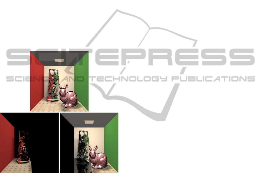
Figure 4: The bottom images show the geometry split be-

tween two workers. The composite image is on top. Note

how the Buddha reﬂects the left side geometry in the left

image and the right side geometry in the right image. The

actual Buddha mesh data was distributed to the worker on

the left.

5 RESULTS

For testing, we used 2-16 Dell T3500 workstations

with dual-core Intel Xeon W3503 CPUs clocked at

2.4 GHz. Each workstation had 4 GB of system

RAM, a 4 GB swap partition, and was running Cen-

tOS 6. FlexRender consists of around 14,000 lines

of code, mostly C++. We leveraged several popular

open source libraries, including LuaJIT, libuv, Msg-

Pack, GLM, and OpenEXR. We used pfstools for tone

mapping our output images and pdiff for computing

perceptual diffs.

5.1 Test Scene

Our test scene, “Toy Store”, has a geometric complex-

ity of nearly 42 million triangles. The room geometry

is relatively simple, but the toys on the shelves are

unique (non-instanced) copies of the Stanford bunny,

Buddha, and dragon meshes that have been remeshed

from their highest quality reconstructions down to

14,249 faces, 49,968 faces, and 34,972 faces respec-

tively. There are 30 toys per shelf and 42 shelves in

the scene for a total of nearly 1,300 meshes. Approx-

imately one quarter of the meshes are rendered using

a mirrored shader, while the others used a standard

Phong shader. The mirrored shader is what causes

some black pixels in the image due to the scene not

being completely enclosed. The scene consists of

1.09 GB of mesh data and 5 GB of BVH data once

the acceleration structures are built.

We rendered a test image at a resolution of

1024x768 with no subpixel antialiasing, 10 Monte

Carlo samples per light (32 lights in the scene), and

a recursion depth limit of 3 bounces. For discussing

speedups initially, we will focus on the 8-worker case

(8 workers in the image plane decomposition conﬁgu-

ration vs. 8 workers in the FlexRender conﬁguration),

but we will discuss varying cluster sizes in Section

5.6.

5.2 Image Plane Decomposition vs.

FlexRender

In the image plane decomposition case, we consider

8 workers by chopping up the image into several ver-

tical slices, with a different machine responsible for

each slice (see Figure 5). The slices are then reassem-

bled to form the ﬁnal output image.

We report the time for each machine to complete

each phase of rendering (loading the scene, building

the BVH, and rendering its slice of the image) in Ta-

ble 1. The total duration of the render would take

10,061 seconds (the slowest time), because the last

slice is needed before the ﬁnal image can be assem-

bled. We report average times for the image plane

decomposition workers compared to FlexRender for

each of the 3 rendering phases in Table 2 and show

FlexRender’s speedup over the average case of 6.57

times faster. We also report the total render time

(all three phases combined), using the slowest image

plane decomposition worker (time to ﬁnal image).

GRAPP2013-InternationalConferenceonComputerGraphicsTheoryandApplications

160

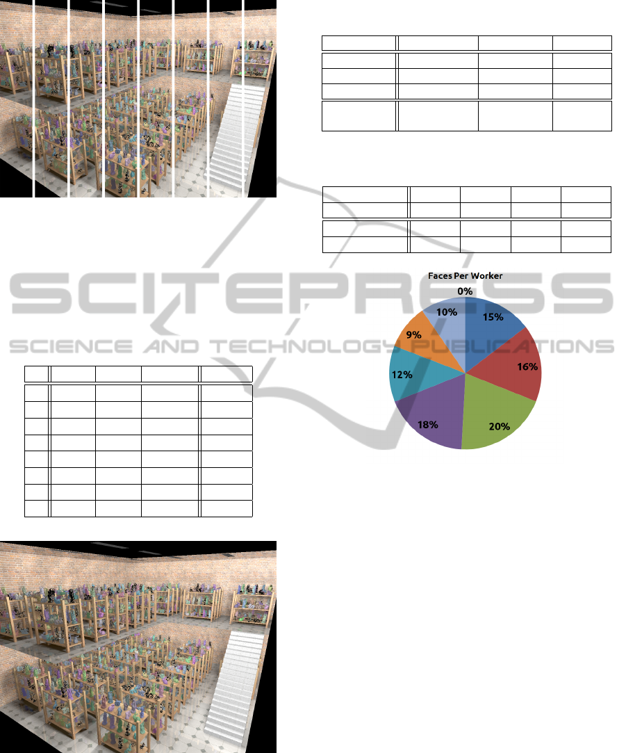
Figure 5: Slices of the Toy Store scene rendered with 8 ma-

chines using image plane decomposition (composite result

image shown in Figure 6).

Table 1: Time for each phase of the IPD algorithm, for each

of the 8 workers, in seconds. These include loading the

scene, building the BVH, rendering the slice, and the total

time of all three phases. Worker 4 was hit particularly hard

with divergent secondary rays, and spent a large amount of

time in I/O wait.

Load BVH Render Total

1 288 169 533 990

2 290 172 1119 1581

3 290 167 1491 1948

4 289 261 9511 10061

5 295 174 1792 2261

6 290 192 677 1159

7 287 167 1109 1561

8 294 171 303 768

Figure 6: Toy Store scene that is comprised of nearly 1,300

meshes and 42 million triangles.

5.3 Geometry Distribution

To ensure the entire scene stays in-core, FlexRen-

der must distribute the geometry across the available

Table 2: Time (in seconds) for each phase of rendering with

FlexRender versus the IPD conﬁguration.

IPD FlexRender Speedup

Loading 290.4 (avg) 326 0.89x

Build BVH 183.6 (avg) 20 9.18x

Rendering 2066.9 (avg) 1186 1.74x

Total 10061 1532 6.57x

(slowest)

Table 3: Percentage of rays that were processed by the given

number of workers.

# of Workers 1 2 3 4

% of Rays 15.8% 25.6% 21.8% 18.8%

# of Workers 5 6 7 8+

% of Rays 8.9% 7.4% 1.5% 0.2%

Figure 7: Percentage of total geometry that was distributed

to each worker. Other than the worker with little geometry

(top corner with only a ﬁll light), the size of geometry per

worker varied from 9% (106 MB of geometry and 488 MB

of BVH data) to 20% (221 MB of geometry 1007 MB of

BVH data) of the entire scene.

RAM in the cluster effectively. With the exception

of one worker, the Morton coding and Z-order curve

did a decent job of partitioning the scene data evenly.

Figure 7 shows a breakdown of the geometry distri-

bution. The one worker which did not contain very

much geometry was in the top corner of the Toy Store

closest to the camera. This octant of the scene only

contained a ﬁll light facing the rest of the geometry.

5.4 Network Hops

The intent of the top-level BVH is to reduce network

cost by only sending rays across the network when

they venture into that worker’s region of space. Since

a BVH exhibits O(log n) traversal, we expect that

with 8 workers rays would be processed by 3 work-

ers in the average case.

Table 3 shows that 63.2% of rays are handled by

3 workers or less, and nearly 16% never even re-

FlexRender:ADistributedRenderingArchitectureforRayTracingHugeScenesonCommodityHardware

161

quire the network. (They are generated on, intersect

with, and are shaded on a single worker.) In addi-

tion, 36.8% of rays must touch more than the expected

3 workers. However, including hops for the corner

cases mentioned in Section 4.4.4, 82% of rays are at

or below O((log n) + 1) and 90.9% of rays are at or

below O((log n) + 2).

5.5 Ray Queue Sizes

Keeping the ray queue size small is critical to the long

term health of the render. If rays begin queuing up

faster than the cluster can process them, eventually

the cluster will begin swapping when accessing rays,

which violates our fundamental performance goal of

staying in-core.

Because of this, we logged ray queue sizes on each

worker over time while rendering Toy Store on a clus-

ter of 16 workers. Figure 8 shows the queue sizes over

time with workers represented as different colors. Ta-

ble 4 breaks down the average queue size, as well as

the maximum size over the course of the entire render

and the storage demands of the maximum size, both

in terms of raw storage space and a fraction of the

system RAM.

Most workers sit comfortably below 1% of their

RAM being used for queued rays, while the busiest

worker used just over 1%. This demonstrates that our

work throttling mechanisms, while simple, are keep-

ing the cluster from generating more work than it can

handle.

Figure 8: Number of rays queued on each worker over time.

Different colors correspond to different workers.

5.6 Cluster Size

To evaluate the scalability of the FlexRender architec-

ture, we ran Toy Store renders with cluster sizes of 4

workers, 8 workers, and 16 workers. For comparison,

we ran the same renders in the image plane decompo-

sition conﬁguration also of 4, 8, and 16 workers.

Table 5 shows a continual and impressive im-

provement in the BVH construction time as the num-

ber of workers increases. This is thanks to the huge

Table 4: Size of ray queues when rendering Toy Store with

a 16-worker FlexRender cluster.

Avg Max Max Memory

Queued Queued Storage Use

1 107 12221 1.49 MB 0.04%

2 506 29796 3.64 MB 0.09%

3 969 34970 4.27 MB 0.10%

4 3116 57597 7.03 MB 0.17%

5 1687 36981 4.51 MB 0.11%

6 1430 44053 5.38 MB 0.13%

7 4070 80899 9.88 MB 0.24%

8 2000 16861 2.06 MB 0.05%

9 3767 97429 11.89 MB 0.29%

10 7921 178191 21.75 MB 0.53%

11 4477 69702 8.51 MB 0.21%

12 4943 92043 11.24 MB 0.27%

13 51164 430736 52.58 MB 1.28%

14 2193 45428 5.55 MB 0.14%

15 0 0 0 MB 0.00%

16 18 1374 0.17 MB 0.01%

Table 5: Comparison of cluster sizes with both image

plane decomposition (IPD) and the FlexRender conﬁgura-

tion (Flex). Times are in seconds.

# of Workers 4 8 16

IPD BVH Build 203 184 171

Flex. BVH Build 39 20 10

Speedup 5.21x 9.20x 17.1x

IPD Render 14833 10061 7702

Flex. Render 1742 1532 970

Speedup 8.51x 6.57x 7.94x

IPD Total 14536 9800 7413

Flex. Total 1405 1206 540

Speedup 10.35x 8.13x 13.73x

parallelization speedup from partitioning the scene

geometry with Morton coding and building each sub-

tree in parallel.

We also see render time improvements of roughly

an order of magnitude, depending on how FlexRen-

der chooses to distribute the geometry based on the

number of workers available. It is likely that this per-

formance advantage will slowly erode at much larger

cluster sizes (due to increasing network communica-

tion costs), but for small to medium cluster sizes we

see approximately linear growth.

5.7 Example Renders

Figure 6 shows the ﬁnal Toy Store scene render, with

nearly 42 million triangles and 1,300 meshes.

Figure 1 shows a scene with even higher resolu-

GRAPP2013-InternationalConferenceonComputerGraphicsTheoryandApplications

162

tion meshes, bringing the geometric complexity up to

87 million triangles, rendered on a cluster of 4 ma-

chines.

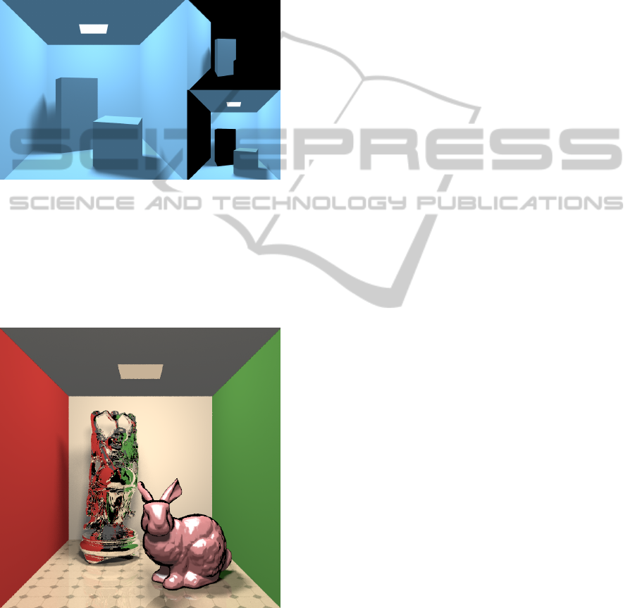
Figure 9 shows a monochromatic Cornell Box ren-

dered by two workers. The ﬁnal composite is on the

left, while the individual image buffers are stacked on

the right. With only direct lighting and no reﬂections,

this clearly shows which geometry was assigned to

each worker.

Figure 9: A monochromatic Cornell Box, showing the dis-

tribution of geometry between two workers.

Figure 10 demonstrates FlexRender’s Lua-based

shader system. The bunny mesh is toon shaded, while

the Buddha mesh has a perfect mirror ﬁnish. Reﬂec-

tion rays for the mirrored Buddha and ﬂoor are cast

directly from the shaders.

Figure 10: A Cornell Box with a toon shaded bunny and

mirrored Buddha.

5.8 Summary

With these results, we have demonstrated that

FlexRender meets our claimed contributions in the

following ways.

• Rays carry enough state to never require replies

thanks to the feed-forward messaging design.

• This design allows the implementation of a shader

system that requires no suspension of shader exe-

cution state as rays are moved between workers.

• FlexRender can correctly and efﬁciently traverse

the scene when workers only contain spatially lo-

cal BVHs, linked by a top-level BVH.

• The system keeps itself regulated and reduces

memory usage by throttling new work generation

and processing rays in an intelligent order.

• FlexRender shows consistent speedups over im-

age plane decomposition, which suffers greatly

from swapping to disk frequently during the ren-

dering process.

5.9 Future Work

FlexRender could beneﬁt from specialized tuning

to scheduling and spatial distribution. Speciﬁcally,

adding dynamic task scheduling as described in

(Navr

atil et al., 2012) could dramatically improve per-

formance, and adopting a more sophisticated spatial

distribution method as described in (Badouel et al.,

1994) could also help with workload distribution.

The cache-oblivious ray reordering technique pre-

sented in (Moon et al., 2010) would complement

our work quite nicely, and could offer another or-

der of magnitude improvement in performance. Ex-

plorations with multiresolution geometry or coupling

FlexRender with existing out-of-core methods would

also dramatically increase the complexity of scenes

FlexRender can handle efﬁciently.

With respect to our existing implementation, some

network hops could be avoided when the ray ﬁn-

ishes traversing the top-level BVH but ends up on a

worker that is not the point of intersection. Because

the worker has no shading assets for the terminating

geometry, it must pass the ray back to the “winning”

worker for shading. By distributing all of the shading

assets (shaders, textures, and materials) to all work-

ers, any worker would be capable of computing shad-

ing regardless of whether it was responsible for the

terminating geometry.

Memory optimizations, such as object pooling,

could exploit the transient nature of many ﬁxed-size

fat rays to reduce allocation overhead and heap frag-

mentation. In addition, the linear BVH node struc-

tures were intentionally padded to 64-bytes to match

the cache line size on current CPUs. However with-

out an aligned STL allocator for the vector that stores

this array of nodes, cache alignment is not guaranteed.

FlexRender:ADistributedRenderingArchitectureforRayTracingHugeScenesonCommodityHardware

163

Additionally, greater code optimization (e.g. use of

SIMD instructions) could also improve performance.

Finally, one of FlexRender’s strengths is that it

decouples the ray tracing computations from shading

with a feed-forward design that requires no replies.

Because messages are both asynchronous and never

return, this opens up the possibility for batching com-

putation to specialized hardware coprocessors, such

as GPUs or the upcoming Intel MIC cards.

REFERENCES

Afra, A. (2012). Interactive ray tracing of large models

using voxel hierarchies. Computer Graphics Forum,

31(1):75–88.

Badouel, D., Bouatouch, K., and Priol, T. (1994). Distribut-

ing data and control for ray tracing in parallel. Com-

puter Graphics and Applications, IEEE, 14(4):69 –77.

Cignoni, P., Montani, C., Scopigno, R., and Rocchini, C.

(1998). A general method for preserving attribute

values on simpliﬁed meshes. In Proceedings of the

conference on Visualization ’98, VIS ’98, pages 59–

66, Los Alamitos, CA, USA. IEEE Computer Society

Press.

Clark, J. H. (1976). Hierarchical geometric models for

visible-surface algorithms. In Proceedings of the 3rd

annual conference on Computer graphics and inter-

active techniques, SIGGRAPH ’76, pages 267–267,

New York, NY, USA. ACM.

Cohen, J., Olano, M., and Manocha, D. (1998).

Appearance-preserving simpliﬁcation. In Proceedings

of the 25th annual conference on Computer graph-

ics and interactive techniques, SIGGRAPH ’98, pages

115–122, New York, NY, USA. ACM.

Dean, J. and Ghemawat, S. (2004). Mapreduce: simpliﬁed

data processing on large clusters. In Proceedings of

the 6th conference on Symposium on Opearting Sys-

tems Design & Implementation - Volume 6, OSDI’04,

pages 10–10, Berkeley, CA, USA. USENIX Associa-

tion.

DeMarle, D. E., Gribble, C. P., and Parker, S. G. (2004).

Memory-savvy distributed interactive ray tracing. In

Proceedings of the 5th Eurographics conference on

Parallel Graphics and Visualization, EG PGV’04,

pages 93–100, Aire-la-Ville, Switzerland, Switzer-

land. Eurographics Association.

Djeu, P., Hunt, W., Wang, R., Elhassan, I., Stoll, G., and

Mark, W. R. (2011). Razor: An architecture for

dynamic multiresolution ray tracing. ACM Trans.

Graph., 30(5):115:1–115:26.

Garanzha, K., Bely, A., Premoze, S., and Galaktionov,

V. (2011). Out-of-core gpu ray tracing of complex

scenes. In ACM SIGGRAPH 2011 Talks, SIGGRAPH

’11, pages 21:1–21:1, New York, NY, USA. ACM.

Hapala, M., Davidovic, T., Wald, I., Havran, V., and

Slusallek, P. (2011). Efﬁcient stack-less bvh traversal

for ray tracing. In 27th Spring Conference on Com-

puter Graphics, SCCG ’11.

Kato, T. and Saito, J. (2002). ”kilauea”: parallel global

illumination renderer. In Proceedings of the Fourth

Eurographics Workshop on Parallel Graphics and Vi-

sualization, EGPGV ’02, pages 7–16, Aire-la-Ville,

Switzerland, Switzerland. Eurographics Association.

Kontkanen, J., Tabellion, E., and Overbeck, R. S. (2011).

Coherent out-of-core point-based global illumination.

In Eurographics Symposium on Rendering.

Krishnamurthy, V. and Levoy, M. (1996). Fitting smooth

surfaces to dense polygon meshes. In Proceedings

of the 23rd annual conference on Computer graph-

ics and interactive techniques, SIGGRAPH ’96, pages

313–324, New York, NY, USA. ACM.

Moon, B., Byun, Y., Kim, T.-J., Claudio, P., Kim, H.-

S., Ban, Y.-J., Nam, S. W., and Yoon, S.-E. (2010).

Cache-oblivious ray reordering. ACM Trans. Graph.,

29(3):28:1–28:10.

Navr

atil, P. A., Fussell, D. S., Lin, C., and Childs,

H. (2012). Dynamic scheduling for large-scale

distributed-memory ray tracing. In Proceedings of Eu-

rographics Symposium on Parallel Graphics and Visu-

alization, pages 61–70.

Northam, L. and Smits, R. (2011). Hort: Hadoop online

ray tracing with mapreduce. In ACM SIGGRAPH

2011 Posters, SIGGRAPH ’11, pages 22:1–22:1, New

York, NY, USA. ACM.

Pantaleoni, J., Fascione, L., Hill, M., and Aila, T. (2010).

Pantaray: fast ray-traced occlusion caching of mas-

sive scenes. In ACM SIGGRAPH 2010 papers, SIG-

GRAPH ’10, pages 37:1–37:10, New York, NY, USA.

ACM.

Reinhard, E., Chalmers, A., and Jansen, F. W. (1999). Hy-

brid scheduling for parallel rendering using coherent

ray tasks. In Proceedings Parallel Visualization and

Graphics Symposium, pages 21–28.

GRAPP2013-InternationalConferenceonComputerGraphicsTheoryandApplications

164