Simple, Fast, Accurate Melanocytic Lesion Segmentation
in 1D Colour Space
F. Peruch
1
, F. Bogo
1
, M. Bonazza
1
, M. Bressan
1
, V. Cappelleri
2
and E. Peserico
1
1
Dip. Ing. Informazione, Univ. Padova, Padova, Italy
2
Dip. Medicina, Univ. Padova, Padova, Italy
Keywords:
Segmentation, Dermatoscopy, Melanoma, Melanocytic Lesion, Naevus.
Abstract:
We present a novel technique for melanocytic lesion segmentation, based on one-dimensional Principal Com-
ponent Analysis (PCA) in colour space. Our technique is simple and extremely fast, segmenting high-
resolution images in a fraction of a second even with the modest computational resources available on a
cell phone – an improvement of an order of magnitude or more over state-of-the-art techniques. Our technique
is also extremely accurate: very experienced dermatologists disagree with its segmentations less than they
disagree with the segmentations of all state-of-the-art techniques we tested, and in fact less than they disagree
with the segmentations of dermatologists of moderate experience.
1 INTRODUCTION
Malignant melanoma is an aggressive form of skin
cancer whose incidence is steadily growing world-
wide (Rigel et al., 1996). Early diagnosis promptly
followed by excision is crucial for patient survival.
Unfortunately, in its early stages malignant melanoma
appears very similar to a benign melanocytic lesion
(a common mole). However, malignant melanoma
can often be recognized even in its early stages by
a trained dermatologist, particularly when observed
through a dermatoscope – an instrument providing
magnification and specific illumination.
The first step in the visual analysis of a
melanocytic lesion is segmentation, i.e. classification
of all points in the image as part of the lesion or of
the surrounding, healthy skin. While segmentation is
typically studied in the context of automated image
analysis, it is a first, necessary step even for human
operators who plan to evaluate quantitative features of
a lesion such as diameter or asymmetry – e.g. in the
context of epidemiological studies correlating those
features to lesion benignity (Stolz et al., 1994).
The most important aspect of a segmentation tech-
nique is accuracy. Accuracy is usually evaluated in
terms of divergence from the segmentation provided
by one or more human “experts”. The most widely
used metric is simply the number of misclassified pix-
els normalized over the size of the lesion (Joel et al.,
2002). A crucial observation is that even expert der-
matologists differ in their assessment of a lesion’s
border (see Figure 1), since lesions are often fuzzy
and there exists no standard operative definition of
whether a portion of skin belongs to a lesion or not
– dermatologists rely on subjective judgement devel-
oped over years of dermatoscopic training. The area
of the disagreement region is typically 10 − 20% of
the area of the lesion itself (Silletti et al., 2009; Bel-
loni Fortina et al., 2011); this is obviously the mini-
mum divergence that an automated system can be ex-
pected to have when evaluated against human experts.
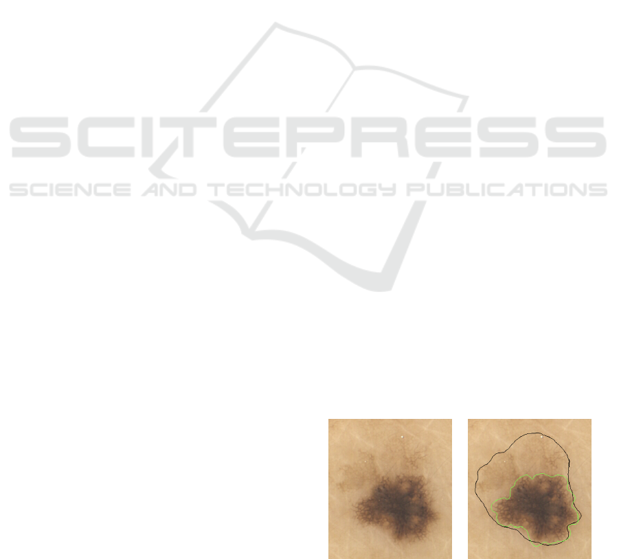
Figure 1: A dermatoscopically imaged melanocytic le-
sion (left) and two widely divergent segmentations obtained
from two experienced dermatologists (right).
The second crucial aspect of an automated seg-
mentation technique is its computational efficiency.
A slow segmentation slows down any system based
on it, meaning such a system cannot be used by a
dermatologist performing real-time diagnosis. This
191
Peruch F., Bogo F., Bonazza M., Bressan M., Cappelleri V. and Peserico E..
Simple, Fast, Accurate Melanocytic Lesion Segmentation in 1D Colour Space.
DOI: 10.5220/0004289601910200
In Proceedings of the International Conference on Computer Vision Theory and Applications (VISAPP-2013), pages 191-200
ISBN: 978-989-8565-47-1
Copyright
c
2013 SCITEPRESS (Science and Technology Publications, Lda.)

is particularly important for hand-held, portable sys-
tems operating with limited computational resources.
This work presents a novel technique for the au-
tomated segmentation of dermatoscopically imaged
melanocytic lesions. Our technique is extremely ac-
curate: very experienced dermatologists disagree with
its results less than they disagree with those of derma-
tologists of moderate experience. It is also extremely
fast, segmenting high-resolution images in a fraction
of a second even with the modest computational re-
sources available on a cell phone – an order of magni-
tude faster than the fastest techniques in the literature.
The rest of this work is organized as follows. Sec-
tion 2 provides a brief review of the state of the art
on melanocytic lesion segmentation. Section 3 intro-
duces our novel approach, based on one-dimensional
Principal Component Analysis (PCA) of the colour
space of the image. Section 4 presents an experimen-
tal comparison of our technique with other segmen-
tation approaches, in terms of accuracy and computa-
tional efficiency. Finally, Section 5 summarizes our
results and discusses their significance.
2 RELATED WORK
Numerous methods have been proposed for lesion
segmentation in dermatoscopic images. According
to a classification commonly adopted in image seg-
mentation (Szeliski, 2010), we can separate them into
three main classes.
The first class aims at identifying lesion bound-
aries by use of edges and smoothness constraints.
A good representative of this class is GVF Snakes
(Erkol et al., 2005). The accuracy in border identifi-
cation may strongly depend on an initial segmentation
estimate, on effective preprocessing (e.g. for hair re-
moval) and on morphological postprocessing (Celebi
et al., 2009; Silveira et al., 2009).
The second class includes “split and merge” tech-
niques. These approaches proceed either by recur-
sively splitting the whole image into pieces based on
region statistics or, conversely, merging pixels and re-
gions together in a hierarchical fashion. Represen-
tatives of this class include Modified JSEG (Celebi
et al., 2007), Stabilized Inverse Diffusion Equations
(SIDE) (Gao et al., 1998), Statistical Region Merg-
ing (SRM) (Celebi et al., 2008), Watershed (Wang
et al., 2010). These algorithms are very sensitive to
correct tuning of a large number of parameters, lead-
ing to highly variable performance (Gao et al., 1998;
Silletti et al., 2009).
The third class of segmentation techniques for
melanocytic lesions discriminates between lesion and
healthy skin on the image’s colour histogram. Af-
ter a preprocessing phase, these approaches classify
each colour as healthy skin or lesional tissue. This
separation is mapped back onto the original image,
from which morphological postprocessing then elim-
inates small, spurious “patches”. Representatives of
this class include Mean-shift (Melli et al., 2006)
and Fuzzy c-means (Schmid, 1999; Cucchiara et al.,
2002; Silletti et al., 2009). Our approach belongs to
this third class.
3 A FIVE-STAGE TECHNIQUE
Our technique proceeds in five stages.
The first stage (Subsection 3.1) is optional and
simply preprocesses the image with an automated hair
removal software. The second stage (Subsection 3.2)
performs a Principal Component Analysis (PCA) of
the colour histogram and reduces the dimensional-
ity of the colour space to 1. The third stage (Sub-
section 3.3) applies a blur filter to the image pro-
jected on the 1D space, in order to reduce noise. The
fourth stage (Subsection 3.4) separates the pixels into
two clusters, segmenting the image into regions cor-
responding to lesional and healthy skin. The fifth and
final stage (Subsection 3.5) morphologically postpro-
cesses the image to remove spurious “patches” and to
identify lesional areas of clinical interest.
3.1 Preprocessing
The presence of hair represents a common obstacle
in dermatoscopic analysis of melanocytic lesions. Al-
though our approach is relatively resilient to the pres-
ence of hair (see Section 4), in some cases automated
hair removal significantly improves the final result.
Thus, when necessary, we perform automated hair re-
moval with VirtualShave (Fiorese et al., 2011).
3.2 PCA in Colour Space
PCA (Abdi and Williams, 2010) is a standard mathe-
matical tool for statistical analysis of observations in
a multi-dimensional space.
We employ PCA to cluster the colours of the im-
age into two classes according to their projection on
the first principal component of the colour histogram
(where each point in the RGB space has a “mass”
equal to the number of pixels with that colour). Using
only one dimension runs against the common wisdom
of melanocytic lesion segmentation through PCA: all
work in this area suggested one should use not only
VISAPP2013-InternationalConferenceonComputerVisionTheoryandApplications
192

the first, but also the second principal component of
the colour histogram.
In practice, we perform PCA on an m-pixel RGB
image in four steps. First, we compute the mean R,
G and B values of the image – the barycentre of the
colour histogram. Then, we compute the 3 × 3 au-
tocorrelation matrix C = M
T
M, where the i
th
row
m
i
= hr
i
g
i
b
i
i of the m × 3 matrix M represents the
three colour components of the i
th
pixel, each compo-
nent normalized by subtracting the mean value of that
colour in the image. Effectively we have:
C =
∑
i
m
i
T
m
i
(1)
so that C can be easily computed by “streaming” the
image pixel by pixel, subtracting the mean R, G, and
B values, computing the 6 distinct products of the
pixel’s colour components, and adding each of those
products to the corresponding product for all other
pixels (note that C is characterized by 6 elements
rather than 9 since it is symmetrical).
Then, we compute the eigenvectors of C and take
the dominant one, i.e. the first principal component
of M. This takes a negligible amount of time since
it only requires computing the roots of a 3
rd
degree
polynomial (the characteristic polynomial of C) and
inverting a 3× 3 matrix.
Finally, we project each row of M onto the princi-
pal component obtaining a one channel grayscale im-
age. Again, this can be achieved by “streaming” the
image and performing only a few arithmetic opera-
tions for each pixel. Thus, the cost of the whole pro-
cedure is essentially that of scanning the image from
main memory three times (once for the average, once
for the covariance, once for the projection).
We noticed an extreme similarity between the
dominant eigenvectors of different melanocytic lesion
images. In a set of 60 images of different lesions from
different patients, for any pair of dominant eigenvec-
tors v and u, we found |v · u| > 0.99.
We then decided to experiment with a simplified
version of our technique, where instead of comput-
ing all eigenvectors of each image, one simply takes
the (precomputed) average of the first eigenvector of
a small “training set” of images. Throughout the rest
of the article, we refer to this simplified version as
static 1D-PCA. Section 4 shows that this crude ap-
proximation still yields surprisingly good results and,
by completely bypassing the PCA portion of the com-
putation, allows significant speedups.
Static 1D-PCA has another important advantage.
Since the 1D colour space on which the image is pro-
jected is independent of the image, one could utilize
the simplified technique with (cheaper) grayscale im-
age acquisition equipment paired with an appropri-
ately tuned (physical) colour filter. This could allow
considerable cost savings when developing biomedi-
cal equipment to e.g. evaluate size, growth patterns or
asymmetry of melanocytic lesions.
3.3 Noise Reduction
In order to reduce noise, we blur the grayscale im-
age corresponding to the projection on the first princi-
pal component. More precisely, we replace the value
of each pixel with the average colour in the 11 × 11
pixel square surrounding it. This filter provides re-
sults comparable to those of a Gaussian filter, but is
far more computationally efficient, requiring a single
scan of the image and no floating point operations.
3.4 Colour Clustering
Operating on the colour histogram h(·) that associates
to each colour c the number of pixels h(c) of that
colour, we separate colours (and thus pixels) into two
clusters corresponding respectively to healthy skin
and lesional tissue. This stage can be divided into a
preprocessing phase and two main phases.
The preprocessing applies to the histogram a
square root operator, followed by a moving average
operator over a window of 11 points. More precisely,
we have:
h
0
(x) =
p
h(x) h
00
(x) =
1
11
x+5
∑
y=x−5
h
0
(y) (2)
The square root operator enhances smaller val-
ues, which is useful when the percentages of healthy
skin and lesional tissue differ widely. The averaging
smooths out small fluctuations.
The second phase clusters colours in two steps.
First we find the positions M
`
,M
s
of two local max-
ima in h
00
(·) that can be assumed as “centres” of, re-
spectively, the lesion cluster and the healthy skin clus-
ter. Then, we determine a frontier point F ∈ [M
`
,M
s
]
separating the two clusters in the histogram.
The position M
1
of the first cluster centre corre-
sponds to the position of the global maximum in h
00
(·)
(see Figure 2). This cluster cannot be classified as le-
sion or healthy skin until the second centre position
is found: lesion area may be larger or smaller than
healthy skin area. The second cluster centre M
2
is
computed as:
M
2
= argmax
x
h
00
(x)(h
00
(M
1
) − h
00
(m
x
))
, x 6= M
1
(3)
where h
00
(m
x
) is the minimum of h
00
(·) between x
and M
1
. The two terms in the product being max-
imized (h
00
(x) and h
00
(M
1
) − h
00
(m
x
)) are meant to
Simple,Fast,AccurateMelanocyticLesionSegmentationin1DColourSpace
193
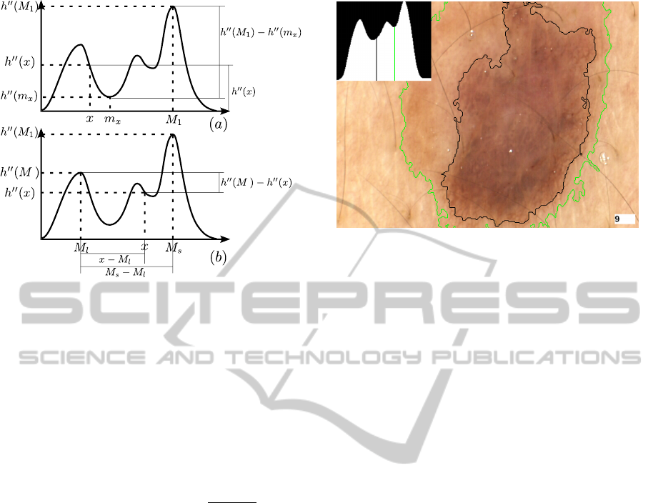
2
2
Figure 2: Identification of clusters centres M
`
and M
s
in the
colour histogram.
favour, in the choice of M
2
, a colour that is “well-
represented” (yielding a high h
00
(x)) and at the same
time is “sharply separated” from M
1
(yielding a high
h
00
(M
1
) − h
00
(m
x
)). Remembering that lesional skin is
darker than healthy skin, M
`
and M
s
are then:
M
`
= min(M
1
,M
2
), M
s
= max(M
1
,M
2
) (4)
Finally, we choose the separation point between
skin colour and lesion colour as:
F = argmax
x
h
00
(M
2
) − h
00
(x)
x − M
`
M
s
− M
`
γ
(5)
where γ ∈ R
+
is the single “tuning” parameter of our
technique – the smaller γ, the “tighter” the segmenta-
tions produced. Informally, the first term in the prod-
uct favours, as a separation point, a colour that is not
well-represented and that thus yields a sharp sepa-
ration between the two clusters. The second term,
whose weight grows with γ, favours a colour closer
to that of healthy skin; this attempts to reproduce the
behaviour of human dermatologists, who tend to clas-
sify as lesion regions of the image that are slightly
darker than the majority of the healthy skin, even
when those regions are considerably lighter than the
“core” of the lesion. Figure 3 illustrates how the clus-
tering results vary as γ increases from 0.8 to 1. On
our dataset, we obtained good results for all values of
γ in [1,1.4]. Note that the fractional exponentiation in
equation 5 is carried out at most once for each of the
256 points of the colour histogram, incurring an over-
all computational cost that is virtually negligible (see
Section 4).
Figure 3: Identification of the separation point between
skin colour and lesion colour for γ = 1 (green) and γ = 0.8
(black). Higher values of γ favour colours closer to that of
healthy skin.
3.5 Postprocessing
Mapping the segmentation from colour space back
onto the original image produces a binary mask,
where each pixel is classified as lesional or healthy.
The postprocessing stage makes this classification
more accurate. First, it corrects several local artefact
“patches” due to a pixel in the image being slightly
darker or lighter than its neighbours. Second, it iden-
tifies all the connected components that, although
classified as healthy, are entirely surrounded by le-
sional pixels; these components usually correspond to
large air bubbles or regressions in a pigmented lesion,
and should therefore be classified as lesional.
Our postprocessing involves two phases (see Fig-
ure 4). We first “downsample” the image in order to
easily identify the boundaries of each lesional compo-
nent through a simplified (and faster!) version of the
technique described in (Suzuki et al., 2003). Then,
we remove all boundaries delimiting connected com-
ponents that are “too small”. We now describe each
phase in greater detail.
Denote by p
i j
the pixel located at row i and col-
umn j in an image, and by v(p
i j
) its value. For any
pixel, we consider its 4-way and 8-way neighbour-
hood – informally, the 4 pixels adjacent to it hori-
zontally or vertically, and the 8 pixels adjacent to it
horizontally, vertically or diagonally. More formally,
for each internal (i.e. non-edge and non-corner) pixel
p
i j
of an image:
Definition 1. The 4-way neighbourhood of p
i j
con-
sists of the 4 pixels p
kl
such that |i − k| + |l − j| = 1.
Definition 2. The 8-way neighbourhood of p
i j
con-
sists of the 8 pixels p
kl
6= p
i j
such that |i − k| ≤ 1 and
|l − j| ≤ 1.
VISAPP2013-InternationalConferenceonComputerVisionTheoryandApplications
194
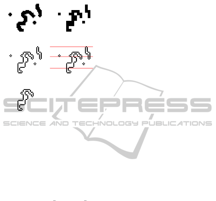
(a) (b)
(c) (d)
(e)
Figure 4: The postprocessing stage. (a) Initial binary mask.
(b) Binary mask after downsampling. (c) Boundary pix-
els. (d) D-rows. (e) Single boundary encircling “sufficient”
area.
We deal with pixels on the edges or corners of the
image by surrounding the image with a 1-pixel-wide
strip of non-lesional pixels so that the pixels of the
original image correspond to the internal pixels of the
expanded image.
In the downsampling phase, we partition the (ex-
panded) image into boxes of 3 × 3 pixels; each pixel
in a box takes the value of the central pixel in the box:
v(p
i j
) , v(p
kl
) with k = 3
i
3
+ 1 , l = 3
j
3
+ 1
(6)
Then, we identify the boundary pixels in the image:
Definition 3. A boundary pixel is a lesional pixel
whose 4-way neighbourhood contains exactly 3 le-
sional pixels.
It would be tedious but straightforward to ver-
ify that, due to the downsampling phase, the 8-way
neighbourhood of any boundary pixel contains ex-
actly 2 boundary pixels.
If we consider any boundary pixel as a vertex of
degree 2 connected by an edge to its two adjacent
boundary pixels, then we obtain a set of disjoint cy-
cle graphs in the image, corresponding to the actual
boundaries of all (putative lesional) connected com-
ponents. This makes it extremely easy to “walk” a
boundary, starting from any of its pixels, following
the edges between adjacent vertices. Note that, up
to this stage, no explicit label has been assigned to
any pixel since those satisfying the boundary defini-
tion are simply marked as “boundary pixels” without
any distinction between different contours; this is the
crucial simplification of our scheme compared to that
of (Suzuki et al., 2003).
In the second step, we compute the area of all con-
nected components of “sufficient” height – we can ex-
pect a minimum height for any lesion of clinical inter-
est of 5% of the image’s height. More formally:
Definition 4. Consider an image of r rows, numbered
from 1 to r starting from the top, and a parameter
d (1 ≤ d ≤ r). We say the i
th
row is a d-row if i
mod d = 0.
Only boundary pixels belonging to a d-row serve
as “starting points” to follow the corresponding
boundary. From the boundary, we can easily obtain
the area of the connected component, as follows. Let
b
i
be the i
th
boundary pixel of the connected compo-
nent on a generic row; then the pixels of the connected
component in that row are those between any two con-
secutive boundary pixels b
i
and b
i+1
with i odd.
Every component with height at least d is
“caught” by our technique, while smaller components
may be missed (if no d-row intersects them) – but
these “small” components are of no interest to us.
d-rows allow considerable speedups as long as d is
larger than 5− 10; while d values equal to (or smaller
than) 5% of the image’s height catch all lesions of
clinical interest. Thus, we set d as 5% of the image’s
height.
In the last step, all boundaries delimiting areas
smaller than one fifth that of the largest connected
component are removed. This takes care of both small
dark patches in healthy skin, and small light patches
within a lesion.
Note that, even if there are many known tech-
niques to identify connected components in a binary
image (Chang et al., 2004; Park et al., 2000; Martin-
Herrero, 2007), they are not suitable for our purposes.
Classic techniques (Chang et al., 2004; Park et al.,
2000) are in general computationally expensive, re-
quiring at least two scans of the image and/or the in-
troduction of additional data structures; in contrast,
our technique requires a single sequential pass plus a
small number of additional accesses to a limited num-
ber of image pixels. Even the optimized, single-pass
approach of (Martin-Herrero, 2007) requires approx-
imately 30% more time than ours; and requires addi-
tional effort to “match” portions of the lesion or of the
skin that do not belong to the same connected compo-
nent.
Simple,Fast,AccurateMelanocyticLesionSegmentationin1DColourSpace
195
4 EXPERIMENTAL EVALUATION
We evaluated our segmentation technique by compar-
ing it to three different state-of-the-art techniques. Af-
ter briefly describing our experimental setup (Subsec-
tion 4.1), we present the evaluation results in terms
of both accuracy (Subsection 4.2) and computational
efficiency (Subsection 4.3).
4.1 Experimental Setup
60 images of melanocytic lesions were acquired at
768 × 576 resolution using a Fotofinder digital
dermatoscope (FotoFinder Systems Inc., 2012). 12
copies of each image were printed on 13cm × 18cm
photographic paper. A copy of each image and a spe-
cial marker pen were given to each of 4 “junior”, 4
“senior” and 4 “expert” dermatologists (having re-
spectively less than 1 year of experience, more than 1
year but no dermatoscopic training, more than 1 year
and dermatoscopic training). Each dermatologist was
then asked to independently draw with the marker the
border of each lesion. The images (and borders) were
scanned and realigned to the same frame of reference.
Finally, the contours provided by the markers were
extracted and compared. This allowed the identifica-
tion, for each pixel of each original image, of the set
of dermatologists classifying it as part of the lesion or
of the surrounding, healthy skin.
We developed a Java implementation of our seg-
mentation technique. In order to evaluate its effi-
ciency on a wide range of devices, from desktops to
hand-helds, we tested it on three different platforms:
a Samsung Galaxy S cell phone with a 1 GHz ARM
Cortex A8 processor, an ASUS Transformer Prime
tablet with a 1.3 GHz Nvidia Tegra 3 processor, and a
desktop PC with a 3.07 GHz Intel Core i7-950 proces-
sor. To provide a clearer evaluation of the strengths
and limitations of our technique, none of our tests
made use of the optional digital hair removal phase
(see Subsection 3.1).
We compared our technique with three differ-
ent state-of-the-art approaches, selecting a represen-
tative technique for each of the three classes in-
troduced in Section 2. We chose techniques with
publicly available implementations. For the first
class, we considered the EdgeFlow algorithm (Ma
and Manjunath, 2000) (http://vision.ece.ucsb.
edu/segmentation/edgeflow/software). Recent
work (Celebi et al., 2009; Silveira et al., 2009) has
already shown how simple active contours methods
(like GVF Snakes) perform quite poorly in terms of
accuracy; we therefore chose to test a method, like
EdgeFlow, which aims at detecting edges more ro-
bustly – unifying the active contour model with tex-
ture segmentation techniques. For the second class,
we tested the Statistical Region Merging (SRM) algo-
rithm (Celebi et al., 2008). For the third class, we
implemented a Java version of the 2D-PCA algorithm
proposed in (Silletti et al., 2009).
SRM does not work properly on lesions adjacent
to the image’s borders. Thus, for its evaluation, we re-
moved from our dataset all such images, testing it on a
reduced dataset of 40 images. Our own technique pro-
duces more accurate segmentations on this reduced
dataset than on the full one (see Subsection 4.2) so
we effectively gave SRM an advantage by allowing it
to run on an “easier” dataset.
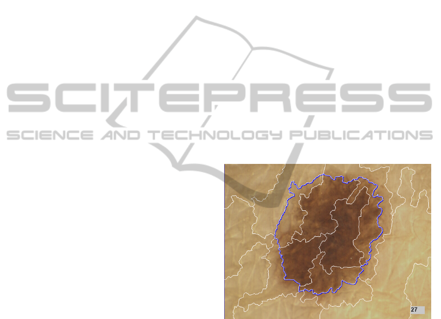
EdgeFlow produces a set of segmented regions,
but does not include a decisional step to determine
which regions should be marked as part of the lesion.
Again, we chose to make the comparison as biased as
possible against our own technique, allowing Edge-
Flow a perfect, instantaneous decisional step. More
precisely, we assumed the decisional step would take
zero time, and would choose as output for EdgeFlow
the set of regions maximizing the segmentation accu-
racy (see Figure 5 and the following Subsection).
Figure 5: Melanocytic lesion segmentation using Edge-
Flow. White contours identify the output of the algorithm.
Blue contours identify the area considered lesional in our
evaluation of EdgeFlow.
4.2 Accuracy
We measured the accuracy of a generic segmenta-
tion S by comparing it to a “ground truth” reference
segmentation R, and counting the number TP of true
positive pixels (classified as lesion by both segmen-
tations), the number FP of false positive pixels (clas-
sified as lesion by S but not by R), the number FN
of false negative pixels (classified as lesion by R but
not by S) and the number TN of true negative pix-
els (classified as lesion by neither segmentation). We
VISAPP2013-InternationalConferenceonComputerVisionTheoryandApplications
196
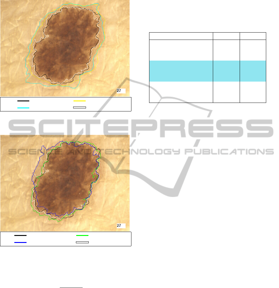
Expert Senior
Junior 1D-PCA
Figure 6: Melanocytic lesion segmentation performed by
human dermatologists and 1D-PCA.
Expert SRM
EdgeFlow 1D-PCA
Figure 7: Melanocytic lesion segmentation performed by
expert dermatologists, SRM, EdgeFlow and 1D-PCA.
then computed the divergence of S from R as:
d
s
=
FP + FN
T P + FN
i.e. as the ratio between the area of the misclassi-
fied region (FP+FN) and the area of the lesion itself
according to the ground truth reference segmentation
(TP+FN) (Hance et al., 1996).
We evaluated the different techniques by compar-
ing their segmentations with those produced by the
4 expert dermatologists (see Table 1). 1D-PCA ob-
tained, on average, a 12.35% divergence from expert
dermatologists. In the spirit of (Silletti et al., 2009),
we also evaluated the 4 senior and 4 junior derma-
tologists using as ground truth the segmentations pro-
duced by the 4 expert dermatologists, and each expert
Table 1: Divergence d
s
(average and standard deviation)
from expert dermatologists in the segmentation performed
by different dermatologists and automated techniques. For
the SRM algorithm, results refer to the reduced dataset (40
images).
Group d
s
(avg) d
s
(std)
Experts 10.40% 6.86%
Seniors 13.57% 9.54%
Juniors 17.24% 15.53%
1D-PCA 12.35% 6.98%
1D-PCA static 12.45% 7.16%
1D-PCA static w/o NR 13.44% 8.21%
2D-PCA 15.58% 7.19%
SRM 15.15% 8.65%
EdgeFlow 16.75% 8.06%
dermatologist using as ground truth the segmentations
produced by the remaining 3 expert dermatologists.
The average divergence of junior dermatologists from
the experts, of the senior dermatologists from the ex-
perts, and of the experts from the other experts, was
respectively 17.24%, 13.57% and 10.40%.
Thus, our 1D-PCA technique achieved a disagree-
ment with expert dermatologists that was lower than
that achieved by junior and senior dermatologists, and
very close to the disagreement of expert dermatolo-
gists between themselves (see Figure 6). This makes
it essentially optimal in terms of accuracy, since dis-
agreement between experts can be viewed as an in-
trinsic, inevitable level of “noise” in the evaluation of
melanocytic lesion border (Silletti et al., 2009).
Quite surprisingly, we observed that some simpli-
fications applied to 1D-PCA lead to only modest re-
ductions in accuracy. Using the simplified static 1D-
PCA (Section 3.2) resulted in a negligible 0.1% loss
in accuracy; eliminating the noise reduction step (see
Subsection 3.3) similarly produced a very small loss
in accuracy – only 1% (see Table 1). As we shall
see in the following Subsection, these small accuracy
losses can be traded for fairly significant speedups.
All other automated techniques exhibited worse
accuracy. EdgeFlow provided the worst results, with
an accuracy comparable to that of junior dermatol-
ogists, despite our “generous” evaluation which, for
each image, considered lesional the set of regions
minimizing divergence from the ground truth (see
Subsection 4.1). The accuracy of SRM, too, was
worse than that of senior dermatologists, again de-
spite a “generous” evaluation on the easier, reduced
dataset (by means of comparison, our technique im-
proved its divergence from 12.35% to 11.87% when
moving from the full dataset to the reduced one). Per-
haps most surprisingly, even 2D-PCA was less accu-
rate than 1D-PCA; this difference may be due in part
to the fact that the second principal component intro-
Simple,Fast,AccurateMelanocyticLesionSegmentationin1DColourSpace
197
duces more noise than information, and in part to the
fact that operating on a 1D colour histogram allows
one to take a slightly more sophisticated approach
to the identification of the colour cluster centres and
boundaries.
As a final note, we remark that our technique
is also extremely robust. Many of the photographs
exhibited a number of defects making segmentation
harder. 1D-PCA is surprisingly resistant to minor im-
perfections like small air bubbles in the anti-reflective
gel or shadows cast by the dermatoscope; we ob-
served an average divergence of only 11.09% on these
images (12 in total). However, images with many pix-
els occluded by dark hair, with large air bubbles cast-
ing deep shadows, or with incorrectly framed lesions
“overflowing” from the image, lead to larger diver-
gences (15.36% on average, on a total of 14 such im-
ages). While digital hair removal (Fiorese et al., 2011)
is a solution to the first problem, the latter two clearly
stress the importance of taking good photographs in
the first place.
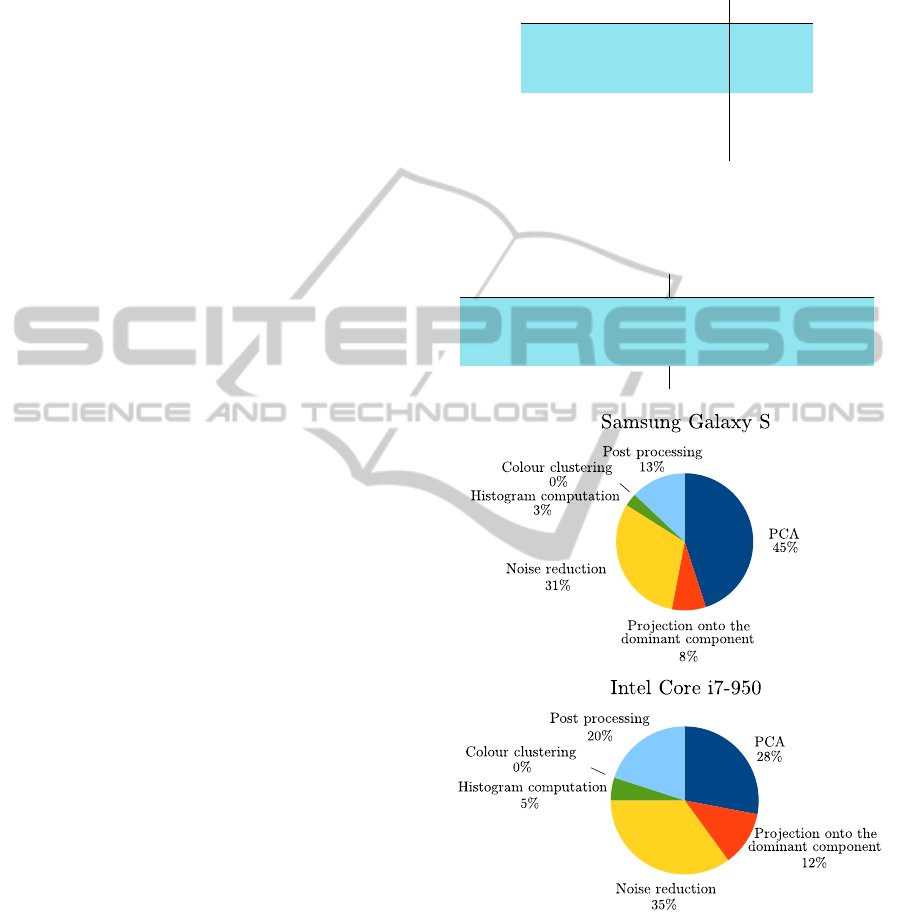
4.3 Computational Resources
Our segmentation technique is extremely fast. Seg-
menting any one of our test images in memory took
less than 0.02 seconds on the Core i7 desktop and
only 0.7 seconds on the Galaxy S cell phone (this
does not account for the possible cost of preprocess-
ing with a hair-removing tool).
Tables 2 and 3 show how the execution time can be
further trimmed down by skipping some computation-
intensive operations that do not significantly improve
the accuracy of the segmentation.
Static 1D-PCA required 30% less execution time
than 1D-PCA – while providing virtually identical
accuracy. Devices with lower computational power
benefit even more from this simplification: on the
the Galaxy S static 1D-PCA required 45% less time
than 1D-PCA. Similarly, skipping the noise reduc-
tion phase (and thus worsening accuracy by a mod-
est 1%) reduced execution time by 30 − 40% (and
by 50 − 55% in the case of static 1D-PCA). Figure
8 summarizes the computational costs of each phase.
In contrast with the (1D and 2D) PCA implemen-
tations, which are written in Java for portability, SRM
and EdgeFlow are written in C (generally more effi-
cient). Thus, we could test them only on the Core i7
platform (see Table 2). 1D-PCA outperformed both
SRM and 2D-PCA by over an order of magnitude in
terms of running time; and EdgeFlow by several or-
ders of magnitude (even though we “charged” Edge-
Flow no time costs for the choice of the lesional re-
gion set – see Subsection 4.1).
Table 2: Execution time in milliseconds of 1D-PCA, static
1D-PCA with and without noise reduction, 2D-PCA, SRM
and EdgeFlow on a desktop PC mounting an Intel Core i7-
950 processor.
Core i7
1D-PCA 17
1D-PCA static 12
1D-PCA static w/o NR 7
2D-PCA 199
SRM 189
EdgeFlow 104789
Table 3: Execution time in milliseconds of 1D-PCA, static
1D-PCA with noise reduction disabled or enabled and 2D-
PCA on a Samsung Galaxy S cell phone and on an ASUS
Transformer Prime tablet.
Galaxy Transformer
1D-PCA 733 411
1D-PCA static 407 286
1D-PCA static w/o NR 185 120
2D-PCA 5986 2778
Figure 8: Time cost breakdown of our technique on a Sam-
sung Galaxy S cell phone and on a desktop PC mounting an
Intel Core i7-950 processor.
The main reason for the extreme computational
performance of 1D-PCA is the fact that the 1D colour
histogram can be processed extremely quickly: only a
handful of simple operations are required for each of
its 256 points, without any need of costly iterations.
And since PCA, colour histogram creation, and mor-
phological postprocessing all boil down to “stream-
VISAPP2013-InternationalConferenceonComputerVisionTheoryandApplications
198

ing” the image while performing a few simple opera-
tions on each of its pixels, the total cost of segmenting
the image is essentially that of scanning it a few times.
5 CONCLUSIONS
Our simple technique for melanocytic lesion segmen-
tation is extremely fast. A Java implementation of it
can segment a large dermatoscopic image in the time
required to simply scan the image a handful of times –
a fraction of a second even on hand-held devices with
modest computational resources. This represents an
improvement of an order of magnitude or more over
state-of-the-art techniques.
At the same time, our technique does not sacrifice
accuracy. It appears more accurate than state-of-the-
art techniques. Perhaps more importantly, it appears
almost as accurate as any segmentation technique can
be, since expert dermatologists disagree with it only
slightly more than they disagree between themselves
– and less than they disagree with dermatologists of
little, or even moderate, experience.
Finally, our technique is extremely robust. It does
not require careful hand-tuning; a single parameter
controls how “tight” the segmentation is. It tolerates
very well small photographic defects, such as small
air bubbles or uneven lighting. It is only slightly less
robust in the face of hair (which could be easily re-
moved, physically or through digital preprocessing),
larger air bubbles, or improper lesion framing. In fact,
our technique is so robust that one can achieve almost
as accurate results with a crude simplification of it
which, instead of projecting the colour space of each
image onto its principal component, projects it onto a
precomputed space independent of the image – allow-
ing even faster processing, as well as use of (cheaper)
monochromatic image acquisition equipment.
ACKNOWLEDGEMENTS
This work was supported by Univ. Padova un-
der strategic project AACSE. F. Peruch, F. Bogo,
M. Bressan and V. Cappelleri were supported in part
by fellowships from Univ. Padova. The authors would
thank the Dermatology Unit of Univ. Padova for its
invaluable help.
REFERENCES
Abdi, H. and Williams, L. J. (2010). Principal component
analysis. WIREs Comp. Stat., 2(4).
Belloni Fortina, A., Peserico, E., Silletti, A., and Zattra, E.
(2011). Where’s the naevus? Inter-operator variability
in the localization of melanocytic lesion border. Skin
Res. and Tech., 18(3).
Celebi, M. E., Aslandogan, Y., and Van Stoecker, W.
(2007). Unsupervised border detection in dermoscopy
images. Skin Res. and Tech., 13(4).
Celebi, M. E., Iyatomi, H., Schaefer, G., and Stoecker, W. V.
(2009). Lesion border detection in dermoscopy im-
ages. Comput. Med. Imaging Graph., 33(2).
Celebi, M. E., Kingravi, H. A., Iyatomi, H., Aslandogan,
Y. A., Van Stoecker, W., Moss, R. H., Malters, J. M.,
Grichnik, J. M., Marghoob, A. A., Rabinovitz, H. S.,
and Menzies, S. W. (2008). Border detection in der-
moscopy images using statistical region merging. Skin
Res. and Tech., 14(3).
Chang, F., Chen, C.-J., and Lu, C.-J. (2004). A linear-time
component-labeling algorithm using contour tracing
technique. Comput. Vis. Image Underst., 93(2).
Cucchiara, R., Grana, C., Seidenari, S., and Pellacani, G.
(2002). Exploiting color and topological features for
region segmentation with recursive fuzzy c-means.
Machine Graph. and Vision, 11(2/3).
Erkol, B., Moss, R. H., Stanley, R. J., Van Stoecker, W.,
and Hvatum, E. (2005). Automatic lesion boundary
detection in dermoscopy images using gradient vector
flow snakes. Skin Res. and Tech., 11(1).
Fiorese, M., Peserico, E., and Silletti, A. (2011). Virtual-
Shave: Automated hair removal from digital dermato-
scopic images. In Proc. of IEEE EMBC.
FotoFinder Systems Inc. (2012). Fotofinder dermoscope.
http://www.fotofinder.de/en.html.
Gao, J., Zhang, J., Fleming, M. G., Pollak, I., and Cognetta,
A. B. (1998). Segmentation of dermatoscopic images
by stabilized inverse diffusion equations. In Proc. of
ICIP.
Hance, G. A., Umbaugh, S. E., Moss, R. H., and Stoecker,
W. V. (1996). Unsupervised color image segmentation
with application to skin tumor borders. In Proc. of
IEEE EMBC.
Joel, G., Schmid-Saugeon, P., Guggisberg, D., Cerottini,
J. P., Braun, R., Krischer, J., Saurat, J. H., and Mu-
rat, K. (2002). Validation of segmentation techniques
for digital dermoscopy. Skin Res. and Tech., 8(4).
Ma, W.-Y. and Manjunath, B. S. (2000). EdgeFlow: a tech-
nique for boundary detection and image segmentation.
IEEE Trans. on Image Processing, 9(8).
Martin-Herrero, J. (2007). Hybrid object labelling in digital
images. Machine Vision and Applications, 18(1).
Melli, R., Grana, C., and Cucchiara, R. (2006). Compari-
son of color clustering algorithms for segmentation of
dermatological images. In Proc. of SPIE.
Park, J.-M., Looney, C. G., and Chen, H.-C. (2000). Fast
connected component labeling algorithm using a di-
vide and conquer technique. In Proc. of ISCA 15th
Conference on Computers and Their Applications.
Rigel, D. S., Friedman, R. J., and Kopf, A. W. (1996).
The incidence of malignant melanoma in the United
States: issues as we approach the 21st century. JAAD,
34(5, Part 1).
Simple,Fast,AccurateMelanocyticLesionSegmentationin1DColourSpace
199

Schmid, P. (1999). Segmentation of digitized dermato-
scopic images by two-dimensional color clustering
comparison. IEEE Trans. on Medical Imaging, 18(2).
Silletti, A., Peserico, E., Mantovan, A., Zattra, E., Peserico,
A., and Belloni Fortina, A. (2009). Variability in hu-
man and automatic segmentation of melanocytic le-
sions. In Proc. of IEEE EMBC.
Silveira, M., Nascimento, J., Marques, J., Marcal, A., Men-
donca, T., Yamauchi, S., Maeda, J., and Rozeira, J.
(2009). Comparison of segmentation methods for
melanoma diagnosis in dermoscopy images. Selected
Topics in Signal Processing, 3(1).
Stolz, W., Merkie, T., Cognetta, A., Vogt, T., Landthaler,
M., Bilek, P., and Plewig, G. (1994). The ABCD rule
of dermatoscopy. JAAD, 30(4).
Suzuki, K., Horiba, I., and Sugie, N. (2003). Linear-time
connected-component labeling based on sequential lo-
cal operations. Comput. Vis. Image Underst., 89(1).
Szeliski, R. (2010). Computer vision: algorithms and ap-
plications. Springer.
Wang, H., Chen, X., Moss, R. H., Stanley, R. J., Stoecker,
W. V., Celebi, M. E., Szalapski, T. M., Malters, J. M.,
Grichnik, J. M., Marghoob, A. A., Rabinovits, H. S.,
and Menzies, S. W. (2010). Watershed segmentation
of dermoscopy images using a watershed technique.
Skin Res. and Tech., 16(3).
VISAPP2013-InternationalConferenceonComputerVisionTheoryandApplications
200
