Adaptively Simulating Inhomogeneous Elastic Deformation

Sei Imai

, Yonghao Yue

, Bing-Yu Chen

1,2

and Tomoyuki Nishita

The University of Tokyo, Tokyo, Japan

National Taiwan University, Taipei, Taiwan

Keywords:

Deformation, Simulation, Elastic Object, Elasticity Matrix, Inhomogeneous, Adaptive Simulation.

Abstract:

In this paper, we present an adaptive approach for simulating elastic deformation of homogeneous and inho-

mogeneous objects based on continuum mechanics. In typical adaptive simulation approaches, the deforming

elastic object is usually subdivided to form a tree structure on the ﬂy. However, they are not directly applicable

for inhomogeneous elastic deformation, since the elasticity matrix, which describes the stiffness, of each ele-

ment in each resolution is difﬁcult to estimate at runtime. Furthermore, as most multi-resolution approaches,

it is usually required that the stiffness of the object should either be uniform all throughout its body or con-

sist of a collection of uniform parts, otherwise the elasticity matrices for the elements in coarse levels cannot

be determined. Hence, we propose a bottom-up sampling approach to estimate the elasticity matrices for all

elements in all levels based on a given stiffness function. Moreover, the subdivision process is also moved to

the off-line preprocessing stage with the elasticity matrix estimation to reduce the runtime computational cost

while achieving the adaptive simulation by adaptively selecting the simulation level on the ﬂy. Therefore, we

can efﬁciently simulate the deformation of an elastic object even with spatially varying stiffness.

1 INTRODUCTION

Physically-based simulation of soft bodies (or elas-

tic objects), e.g., jelly, is important for movies and

video games. Currently a lot of techniques are car-

ried out in soft body dynamics in computer graph-

ics. Mass-spring- and particle-based models (e.g.,

(Tu and Terzopoulos, 1994; Lee et al., 1995; Baraff

and Witkin, 1998)) are usually used for interactive

applications (e.g., video games), and more accurate

simulation methods based on continuum mechanics

(e.g., by using FEM, or ﬁnite element method) are

mainly used for ﬁlming because they can usually pro-

vide higher accuracy results. Since FEM-based mod-

els require heavy calculation, several multi-resolution

approaches like adaptive subdivision techniques (e.g.,

(Debunne et al., 2001; Grinspun et al., 2002)) are pro-

posed.

In general multi-resolution approaches, the input

elastic object is divided into several elements (in our

case, tetrahedra) which form a hierarchical structure.

That is, several sets of elements representing the ob-

ject are constructed for various resolutions (or levels),

and a tree-like(i.e., parent-children)relationship is es-

tablished between the elements in different levels. A

difﬁculty in using such approaches for simulating in-

homogeneous elastic deformation is that the elasticity

matrices, which describe the stiffness, of the elements

in different levels may have different values, because

a parent element may contain the children elements

with different stiffness. In typical multi-resolution

methods, a parent element shares the elasticity matri-

ces with its children elements, making that the object

needs to either be uniform or consist of a collection

of uniform parts. Moreover, to achieve the adaptive

simulation in the typical methods, the discretization

(i.e., tetrahedron subdivision) is usually performed on

the ﬂy. However, since the elasticity matrix of each

element in each resolution is difﬁcult to estimate at

runtime, it is hard to directly apply such approaches

for inhomogeneous elastic deformation.

In this paper, we present a bottom-up sampling ap-

proach to estimate the elasticity matrices for all el-

ements in all levels based on a given stiffness func-

tion before performing the simulation. Using the pre-

sented approach, a parent element can consist of the

children elements with different or even continuously

varying stiffness. Moreover, the tetrahedron subdivi-

sion is also moved to the off-line preprocessing stage

with the elasticity matrix estimation to ease the run-

time processes while achieving the adaptive simula-

tion by adaptively selecting the simulation level on

the ﬂy.

Our approach is composed from the off-line pre-

237

Imai S., Yue Y., Chen B. and Nishita T..

Adaptively Simulating Inhomogeneous Elastic Deformation.

DOI: 10.5220/0004290302370244

In Proceedings of the International Conference on Computer Graphics Theory and Applications and International Conference on Information

Visualization Theory and Applications (GRAPP-2013), pages 237-244

ISBN: 978-989-8565-46-4

 2013 SCITEPRESS (Science and Technology Publications, Lda.)

soft

hard

stiffness functionbase tetrahedra model

Input

level 0 model level 1 model

Tree Structure Construction

level 0 model level 1 model

Elasticity Matrix Estimation

Preprocessing

adaptive level selection

Simulation

Run-time

force computation model updating

Figure 1: The overview of our adaptive simulation scheme. The illustration is drawn in 2D for simplicity.

processing and runtime stages. During the prepro-

cessing, the input elastic object is ﬁrst recursively

subdivided into several tetrahedra to construct the

multi-resolution tree structure while keeping the qual-

ity of the subdividedtetrahedra as good as possible for

stable simulation. Next, based on the given stiffness

function, the elasticity matrices of all elements (i.e.,

tetrahedra) are estimated from ﬁne levels to coarse

levels through a sampling approach. According to

the bottom-up operation, we can acquire the elasticity

matrices of all elements in all levels. At runtime, the

simulating elements are selected adaptively according

to a user-given error-threshold and the strain posed on

the elements with spatially varying stiffness. By using

our approach, we can simulate the deformation of in-

homogeneous as well as homogeneous elastic objects

adaptively.

2 RELATED WORK

There is a considerable amount of research on elastic

deformation simulation in computer graphics (Gib-

son and Mirtich, 1997; Nealen et al., 2006). Meth-

ods using mass-spring- or particle-based models (Tu

and Terzopoulos, 1994; Lee et al., 1995; Baraff and

Witkin, 1998) are usually used for interactive appli-

cations, such as video games. To obtain more accu-

rate results, one can use the methods that compute the

continuum mechanics. Such methods can be typically

classiﬁed to meshless ones (e.g., (Faure et al., 2011))

and ﬁnite element methods (FEM). In this paper, we

focus on FEM.

FEM divides the space into small regions utilizing

ﬁnite elements like tetrahedra (O’Brien and Hodgins,

1999; M¨uller et al., 2001) or hexahedra (Capell et al.,

2002). To improve FEM, a large amount of research

has been conducted for the discretization of the in-

put object (e.g., (Shewchuk, 1998) or (Schaefer et al.,

2004)), and for accelerating the computation. To re-

duce the heavy computation cost of FEM, adaptive

subdivision approaches (e.g., (Debunne et al., 2001;

Grinspun et al., 2002; Dequidt et al., 2005)) are usu-

ally used. These approaches subdivide the input ob-

ject according to its strain at runtime. A major prob-

lem of such methods is that they can only be applied

to homogeneous objects.

There are also some methods that can simulate in-

homogeneous elastic objects, e.g., (Chentanez et al.,

2009), but are also time-consuming. One of the

speed-up approaches is numerically coarsening the

linear elastic object (Kharevych et al., 2009). In

this method, the inhomogeneousobjects are deformed

with coarsened tetrahedra, and the ﬁne structures are

mapped into the interpolated position. In (Nesme

et al., 2009), the inhomogeneous elastic object is em-

bedded into grids and the grids’ elasticities are com-

puted to achieve inhomogeneous deformation. How-

ever, to the best of our knowledge, there is no adap-

tive approach for simulating inhomogeneous elastic

objects.

3 ADAPTIVE SIMULATION

SCHEME

Our method is an adaptive approach and based on

FEM (O’Brien and Hodgins, 1999). In typical adap-

tive simulation methods, the deforming elastic object

is subdivided adaptively on the ﬂy, which usually re-

quires the material of the object to be as uniform as

possible. Unlike such methods, our adaptive simula-

tion scheme moves the subdivision process to an off-

line preprocessing stage (Sec. 3.1) with the elasticity

matrix estimation (Sec. 4) to reduce the runtime sim-

ulation cost (Sec. 3.2 and Sec. 5) as shown in Fig. 1.

Therefore, our approach is constructed from the off-

line preprocessing stage and the runtime simulation

stage.

3.1 Tree Structure Construction

In our off-line preprocessing stage, we ﬁrst con-

struct the tree structure for the adaptive simulation

scheme while assuming that the input object is al-

ready roughly tetrahedralized

. Based on this input

tetrahedra set, we further recursively subdivide it to

form a tree structure, while keeping the shapes of the

subdivided tetrahedra as “high quality” as possible,

We believe that this assumption could be improved in

the future.

GRAPP2013-InternationalConferenceonComputerGraphicsTheoryandApplications

238

Tet

111

Tet

112

Tet

121

Tet

122

Tet

211

Tet

212

Tet

221

Tet

222

Tet

311

Tet

312

Tet

321

Tet

322

Tet

Tetrahedra front

Base tetrahedra set

Figure 2: Illustration of the tetrahedra tree. The base tetra-

hedra set as the roots is the input tetrahedra set which is also

the coarsest simulation level. Any cut through the interme-

diate tetrahedra forms a speciﬁc simulation resolution.

otherwise the simulation will easily diverge at run-

time. Although there are several tetrahedron subdivi-

sion approaches applicable to this tree structure con-

struction, to guarantee the subdivided elements only

consist of tetrahedra, we used a tetrahedron subdivi-

sion approach like (Liu and Joe, 1995).

3.2 Simulation with Tetrahedra Front

For a given tetrahedra tree, we ﬁrst deﬁne a “tetrahe-

dra front” as shown in Fig. 2, which is a cut through

the intermediate tetrahedra to form a speciﬁc resolu-

tion for simulation and usually used in mesh simpli-

ﬁcation papers (e.g., (Hoppe, 1996)). If the “tetra-

hedra front” contains all leaf tetrahedra, the simu-

lation will be performed in the ﬁnest resolution to

achieve the most accurate simulation result. On the

other hand, once the “tetrahedra front” only contains

the “base tetrahedra set”, the simulation will be per-

formed with only the input tetrahedra set (i.e., in the

coarsest level) to achieve the best simulation perfor-

mance. Hence, before performing the deformation

simulation, we have to ﬁrst decide the “tetrahedra

front” in the tetrahedra tree, in order to maximize the

simulation performance while keeping the simulation

accuracy to achieve the adaptive simulation (detailed

in Sec. 5.2 and Sec. 5.1).

After deciding the tetrahedra front, the object can

be deformed in accordance with the following equa-

tion:

σ = Cε, (1)

which is the Hooke’s law generalized to three-

dimensional case, where σ,ε ∈ R

is the strain and

stress vectors, respectively, and C ∈ R

6×6

is an elas-

ticity matrix which deﬁnes the material (i.e., stiffness)

of the deforming elastic object

In some literature, the strain, stress and elasticity are

described as tensors, which are equivalent to the formu-

lation used in this paper. We used the matrix-vector

form (Zienkiewicz et al., 2005) for simplicity.

In the deformation simulation, we repeat the fol-

lowing process in each time-step. First, we calcu-

late the strain vector ε of each element (tetrahedron).

Next, we calculate the stress vector σ with the elastic-

ity matrix C in accordance with Eq.(1). Then, we cal-

culate the acceleration, velocity and position of each

vertex at that time-step. Finally, we perform a proce-

dure described in Sec. 5.3 to handle T-junctions.

4 ELASTICITY MATRIX

ESTIMATION AND VALID

RANGE

After the tetrahedron subdivision, our tree structure

contains only tetrahedra. If we ﬁnely subdivide the

input elastic object, we can assume that all the tetra-

hedra in the ﬁnest level n (i.e., the leaf tetrahedra)

are nearly uniform, and their elasticity matrices C can

be easily obtained from the given stiffness function

Hence, we then need to estimate the elasticity matri-

ces C of the elements (i.e., tetrahedra) in coarse levels

(i.e., level 0 to n − 1) through a bottom-up sampling

approach.

Remember that an elasticity matrix C describes

the linear relationship between a stress vector σ and a

strain vector ε as shown in Eq.(1). This means that if

we know the stress vector σ given the strain vector ε,

we can compute the elasticity matrix C by solving a

linear equation. Thus, the basic idea of our bottom-up

approach is to ﬁrst move the tetrahedra in the coarse

level according to ε, simulate the deformation in the

ﬁne level, then obtain σ in the ﬁne level and reinter-

pret this σ as the one in the coarse level. Finally, we

can obtain C from the linear relationship between σ

and ε in the coarse level. We describe the details be-

low.

4.1 Strain Vector Decomposition

To make the calculation for solving the linear equa-

tion simple, we ﬁrst decompose the strain vector ε into

six bases as the linear combination form as:

ε =

∑

m=1

(m)

, (2)

where m = 1,...,6 is the index of each base, α

(m)

∈ R

is a scalar ranged in −1 < α

(m)

< 1, and ε

(m)

is one

of the linear isolated strain vector bases, in which the

m-th element is 1 and others are 0.

If this assumption is not valid, we could apply numeri-

cal coarsening to compute the elasticity matrices

AdaptivelySimulatingInhomogeneousElasticDeformation

239

Next, since the Hooke’s law is linear, we can

further decompose Eq.(1) into σ =

∑

m=1

(m)

Cε

(m)

and the j-th element σ

of the vector σ can

be represented as σ

∑

m=1

(m)

∑

k=1

(m)

∑

m=1

(m)

, where C

is one of the elements of

C in the j-th column and k-th row, and ε

(m)

is the k-th

element of ε

(m)

. Alternatively, we have

σ =

∑

m=1

(m)

, (3)

where C

is the m-th row of C.

4.2 Elasticity Matrix Estimation

Based on Eq.(3), to determine the elements of C, for

each row m, we let α

(m)

be nonzero and α

′

)

′

6= m)

be zero, and compute C

as C

= σ/α

(m)

. However,

for accurately computing C

, it is not sufﬁcient to use

only a single value of α

(m)

for the following two rea-

sons. First, σ obtained from the simulation may con-

tain numerical errors. Second, the linear relationship

= σ/α

(m)

is only valid for small deformations,

i.e., when |α

(m)

| is small. Hence, we sample multi-

ple couples of the scalar α

(m)

for each ε

(m)

to esti-

mate C

as shown in Fig. 3. From the estimation, we

also obtain a valid range for α

(m)

such that the linear

relationship is valid (detailed in Sec. 4.3).

To estimate the unknown elasticity matrix of a

tetrahedron in level n − 1 from the known elasticity

matrices of tetrahedra in level n, we ﬁrst, for a base

m, determine a value of α

(m)

and let the strain vector

ε = α

(m)

(i.e., for other bases m

′

6= m, α

′

)

= 0).

Then, the vertices in level n − 1 are moved so that

the strain vector of the parent tetrahedron equals to

the determined strain vector ε. From these vertices,

we initialize the positions of the vertices in level n as

follows. The vertices in level n can be grouped into

1) the vertices which have corresponding vertices in

level n − 1, and 2) the other vertices which do not

have. For the former vertices, we ﬁx their positions to

the locations of their corresponding vertices in level

n− 1. For the latter ones, their positions are allowed

to moveduring the process described later and are ini-

tialized using linear interpolation from the vertices in

level n− 1.

After initializing the positions of the vertices in

level n, we simulate the elastic deformation of the

tetrahedra in level n based on Eq.(1) using the known

elasticity matrices in level n. In this simulation, only

the positions of the vertices that are allowed to move

are updated. After the stresses are balanced, we then

calculate the stress vector σ in level n − 1 from the

-0.4

-0.3

-0.2

-0.1

0.1

0.2

0.3

0.4

0.5

-1.5 -1 -0.5 0 0.5 1 1.5

ﬁ!ed line

sampling data

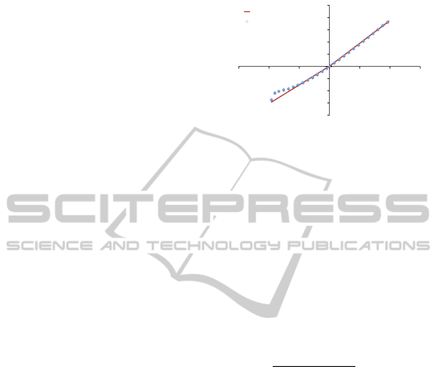
Figure 3: The relationship between α

(m)

(the x-axis) and a

vector component of σ (the y-axis).

stress vectors in level n to obtain one sample of the re-

lationship between a stress vector and a strain vector

as one of the blue dots shown in Fig. 3. By changing

the magnitude of the scalar α

(m)

arbitrarily, we can

obtain multiple samples.

Finally, we can use a straight line to ﬁt the mul-

tiple samples while ignoring some outliers as the red

line shown in Fig. 3, and the slope of the ﬁtted line is

the element of the elasticity matrix of level n− 1.

4.3 Valid Range for Strain Vectors

As described in the previous section, the linear rela-

tionship used for estimating the elasticity matrix is

only valid for small deformations. Hence, the value

of the element C

of the elasticity matrix is valid if

the following condition for α

(m)

is satisﬁed.

|α

(m)

− σ

(α

(m)

|α

(m)

< T

, (4)

where T

is a user-speciﬁed threshold,C

is the slope

of the ﬁtted line as shown in Fig. 3, and σ

(α

(m)

) is

the value obtained from the simulation (i.e., one of the

blue dots in Fig. 3). Using only the above condition,

however, results in erroneous conditioning when the

denominator is small. Thus, we also introduce the

following condition.

|α

(m)

− σ

(α

(m)

)| < T

, (5)

where T

is another user-speciﬁed threshold. If either

of the two above conditions is satisﬁed, we can apply

linear ﬁtting for that range. We denote the lower and

upper bounds of this valid range as α

(m)

min

and α

(m)

max

respectively, and set T

= 1.0× 10

−2

and T

= 1.0 ×

−4

in our experiment.

These two thresholds are the parameters to control

the error bound. If they are set smaller, the allowed

error becomes smaller (i.e., more accurate). Thus, the

valid range will be narrower and the simulation tends

to switch to ﬁner levels more often.

GRAPP2013-InternationalConferenceonComputerGraphicsTheoryandApplications

240

5 ADAPTIVE LEVEL SELECTION

Our runtime operation consists of three steps: 1) up-

dating the tetrahedron front; 2) calculating the inter-

nal force and updating the velocity and position of

each node; and 3) adjusting the vertices aligned at

the T-junctions. In step 1), the tetrahedron front is

updated by either replacing children tetrahedra with

their parent tetrahedron, or replacing a parent tetrahe-

dron with its children tetrahedra. We describe the con-

ditions for these replacements in Sec. 5.1 and Sec. 5.2.

For step 2), please refer to (O’Brien and Hodgins,

1999). Finally, the details of step 3) are described in

Sec. 5.3.

5.1 Coarse to Fine Switching

To decide the tetrahedron front for simulation, we ﬁrst

check if we need to switch a tetrahedron in the tetrahe-

dron front to its children tetrahedra in one ﬁner level

while taking into account the valid range of strain vec-

tor described in Sec. 4.3. For each tetrahedron, we

calculate the strain vector ε posed on the tetrahedron

and decompose it using ε

(m)

as Eq.(2). Then, if all

(m)

are in their valid ranges, i.e., for all m,

(m)

min

< α

(m)

< α

(m)

max

, (6)

we regard the selected level as proper. Otherwise, we

switch this tetrahedron to its children.

5.2 Fine to Coarse Switching

As using a parent (coarse) tetrahedron instead of its

children tetrahedra would introduce errors into the

simulation, switching from ﬁne level to coarse level

needs to be taken carefully, and indeed it is more com-

plex. In our method, we switch to a parent tetrahedron

if the following three conditions are all satisﬁed.

1. The strain vector of the parent tetrahedron is

within the valid range as Eq.(6).

2. All of the children tetrahedra of the parent tetra-

hedron are contained in the tetrahedra front.

3. All strain vectors of the children tetrahedra are al-

most the same as that of their parent tetrahedron.

The ﬁrst condition is needed to ensure that the re-

lationship between the strain and stress vectors can

be accurately handled even when we use the coarse

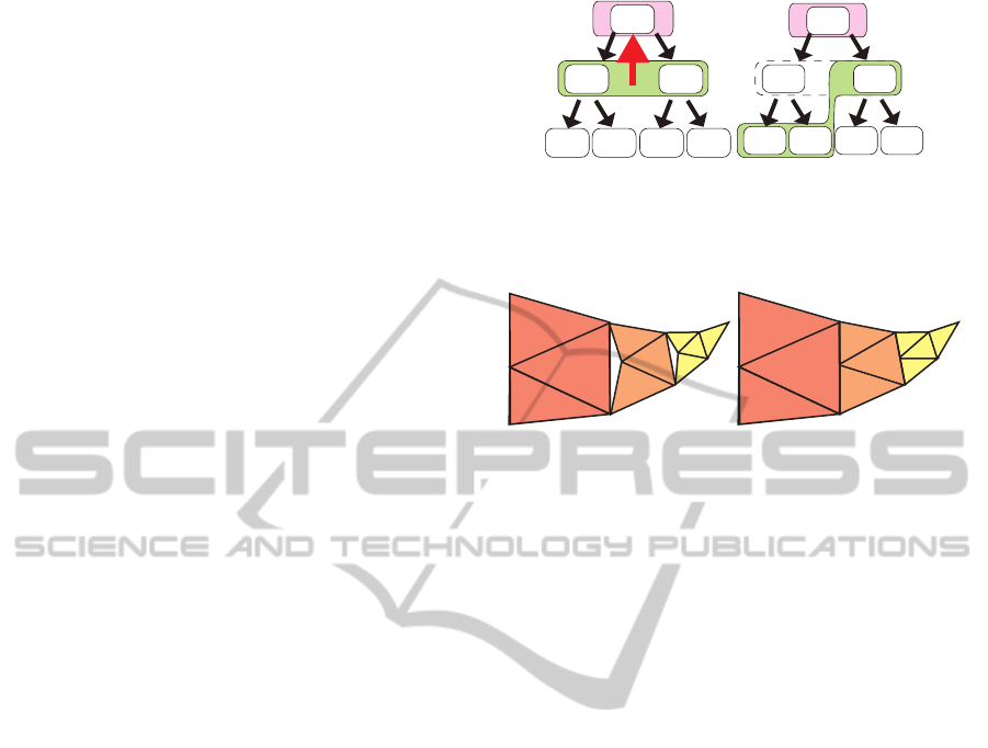
level. The second condition is needed to avoid the

case when ﬁner levels are used to represent one or

more children tetrahedra of the parent tetrahedron, as

shown in Fig.4. In this case, switching to the par-

ent tetrahedron would discard the ﬁne structure which

is needed for a sufﬁciently accurate calculation. The

Tet

111

Tet

112

Tet

121

Tet

122

(a)

Tet

111

Tet

112

Tet

121

Tet

122

(b)

Figure 4: (a) A coarse to ﬁne switchable case and (b) an

unswitchable case. The green area is the tetrahedron front

and pink area is the candidate tetrahedron to switch.

(a) (b)

Figure 5: (a) A crack may appear due to the T-junction prob-

lem. (b) The T-junction vertex of the tetrahedra in the ﬁne

level is ﬁxed at the middle point of its corresponding edge of

the coarse tetrahedron to ensure the continuity of the object.

third condition is needed to take into account the ac-

tual forces posed on the children tetrahedra. If the

forces largely differ across the tetrahedra, then using

the parent tetrahedron would result in a crude approx-

imation of the forces.

5.3 Handling T-junctions

Tetrahedra in different levels may cause a T-junction

problem as shown in Fig. 5. At the T-junction, there

is a T-junction vertex belonging to the tetrahedra in

the ﬁne level, but is not shared by their parent tetra-

hedron in the coarse level, a crack or overlap may

thus occur. To avoid this problem, we enforce the

T-junction vertex to be ﬁxed at the middle point of

its corresponding edge of the coarse tetrahedron like

other adaptive modeling methods. The procedure of

this enforcement is performed from the coarsest level

toward the ﬁnest level.

6 RESULTS

The simulation has been performed on a PC with an

Intel Core X980 3.33 GHz CPU with 8 GB memory.

First, we show the comparison between our ap-

proach and the existing method (O’Brien and Hod-

gins, 1999), by simulating a deforming box, which

is ﬁxed on a wall, according to the gravity force as

shown in Fig. 6. At the beginning of the simula-

tion, the box in our approach was mostly composed

AdaptivelySimulatingInhomogeneousElasticDeformation

241

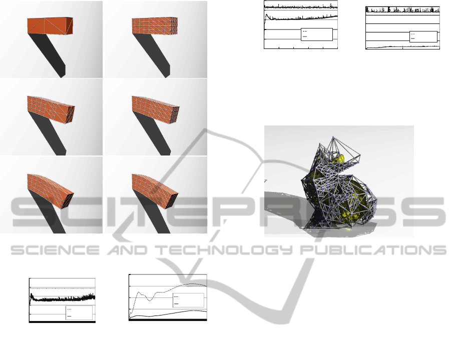
Figure 6: A comparison of our method (left) and the exist-

ing method (right).

200

400

600

800

1000

1 301 601 901 1201

The number of

tetrahedra

Steps

Finest

Adaptive

(a)

0.0%

0.5%

1.0%

1.5%

2.0%

1 301 601 901 1201

Error

Steps

Average

Maximum

(b)

Figure 7: (a) The numbers of tetrahedra of our adaptive ap-

proach (solid line) and of the ﬁnest level (dashed line). (b)

Computation error of our method. Solid line: average error.

Dotted line: maximum error.

of coarse tetrahedra, since the magnitude of the defor-

mation is small for most parts (Fig. 7). A few seconds

later, some parts of the box that moved a lot switched

to a ﬁner level, but the rest parts kept their original

level since the movement is not so large. When the

deformation reached the equilibrium, most parts were

smoothly deformed and the levels they belonged to

were almost the ﬁnest.

We also checked the processing time the defor-

mation requires on each update as shown in Fig. 8.

First, since most tetrahedra belonged to the coarsest

level in the beginning of the simulation, the process-

ing time of our method was an order of magnitude

faster than that of the existing method. As the simula-

tion progressed, the level switched to a ﬁner level and

more processing time was required. When all parts

switched to the ﬁnest level due to the large deforma-

tion, the calculation time was still competitive to the

existing method.

0.5

1.5

2.5

1 301 601 901 1201

Computation time

per step [ms]

Simulation time [sec]

Finest

Adaptive

(a)

0.5

1.5

2.5

0 5 10

Computation time

per step [ms]

Simulation time [sec]

Finest

Adaptive

(b)

Figure 8: (a)A comparison of the calculation time between

using our adaptive approach (solid line) and the ﬁnest level

(dashed line). (b) A zoomed view of (a).

Figure 9: A smooth mesh is embedded in the tetrahedral

structure.

The computation error between using our adap-

tive approach and using the ﬁnest level is shown in

Fig. 7. The error is deﬁned as the difference between

the locations of the vertices when using our adaptive

approach and the ﬁnest level. The error is normalized

by dividing the difference by the longest edge length

of the box. The average of the errors is under 0.5%

and the maximum value of the errors is under 1.7%.

For rendering, we want to acquire a smooth result

with the tetrahedral structure used for simulation as

shown in Fig. 9. During the initial step, for each ver-

tex of the embedded smooth mesh, we compute the

corresponding ﬁnest tetrahedron the vertex belongs

to, and compute the barycentric coordinates of the

vertex in the tetrahedron. During the rendering step,

the location of each vertex of the embedded smooth

mesh is computed from a liner interpolation using the

barycentric coordinates and the locations of the ver-

tices of the corresponding tetrahedron.

To show a more complicated result, we simulated

a bunny-shaped inhomogeneousjelly according to the

gravity force as shown in Fig. 10. The bunny has a

continuous stiffness distribution, so that the (red col-

ored) bottom part is stiff but the (yellow colored) top

part is soft. Because of the inhomogeneous stiffness,

the bunny can stand alone thanks to its stiff feet, while

its ears are hanging down from the head since they are

soft.

We also simulated an armadillo-shaped inhomo-

geneous jelly (Fig. 12). In this example, the gravity

GRAPP2013-InternationalConferenceonComputerGraphicsTheoryandApplications

242

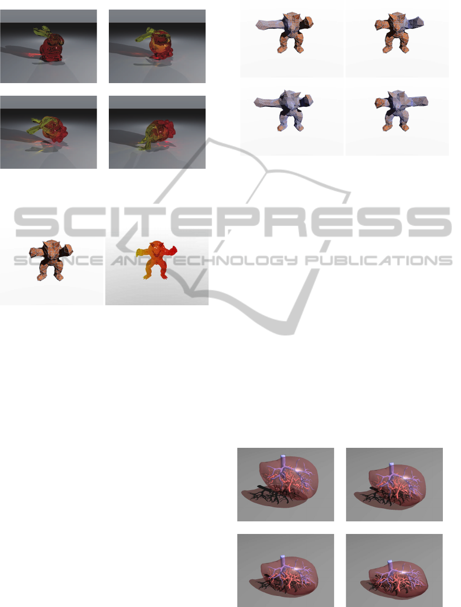
Figure 10: The simulation of a inhomogeneous bunny-

shaped jelly. The stiffness of jelly is continuously different

from bottom to top. The part around its feet is stiff (red) and

the part around its ears is soft (yellow).

Figure 11: Left: the tetrahedra mesh of the coarsest level.

Right: the stiffness is continuously varying from left to

right.

force is not applied. The armadillo has a continuous

stiffness distribution from left to right (again, red and

yellow colors indicate more stiff and soft portions,

see Fig. 11). We applied external forces in the same

magnitude on its right and left hand. Since its right

hand is more soft, with the same magnitude of exter-

nal forces, it gets longer than the left hand.

To show a deformation of an object made of parts

with different stiffness, we simulated the deformation

of an inhomogeneous liver according to the gravity

force as shown in Fig. 13. The vessels are stiffer than

other tissues.

7 CONCLUSIONS AND FUTURE

WORK

We proposed an adaptive approach for simulating

elastic deformation of homogeneous and inhomoge-

neous objects based on FEM. A difﬁculty in using an

adaptive as well as multi-resolution approach for sim-

ulating inhomogeneous elastic deformation is that the

elasticity matrices of the elements in different levels

may have different values, because a parent element

Figure 12: Left column: The force is applied on the right

hand of the armadillo. Right column: The force is applied

on its left hand. Top and bottom rows show the results after

400 and 800 steps, respectively.

may contain the children elements with different stiff-

ness. Thus, we proposed a bottom-up sampling ap-

proach to estimate the elasticity matrices for the ele-

ments in coarse levelsfrom the children elements with

known elasticity matrices, so that a parent element

can consist of the children elements with different or

even continuously varying stiffness. Moreover, unlike

other typical adaptivesimulation methods, which sub-

divided the deforming object adaptively on the ﬂy, we

moved the tedious tetrahedron subdivision to the off-

line preprocessing stage to ease the burden on the run-

time simulation. Furthermore, we presented an adap-

tive simulation scheme, which selects the appropriate

levels on the ﬂy according to the error-threshold given

by the user and the strain posed on the elements.

Our approach is faster than existing method in

processing time in each time-step when coarser levels

are selected. In the worst case, the processing time is

still comparable to that of the existing methods. Since

Figure 13: The simulation of liver. The vessels(blue and

red) is stiffer than the other tissues.

AdaptivelySimulatingInhomogeneousElasticDeformation

243

we can estimate the elasticity matrices in the coarse

levels through a sampling approach, we believe that

we can also compute the viscosity constants in a sim-

ilar way.

REFERENCES

Baraff, D. and Witkin, A. (1998). Large steps in cloth sim-

ulation. In ACM SIGGRAPH 1998 Conference Pro-

ceedings, pages 43–54.

Capell, S., Green, S., Curless, B., Duchamp, T., and

Popovi´c, Z. (2002). A multiresolution framework for

dynamic deformations. In Proceedings of the 2002

ACM SIGGRAPH/Eurographics Symposium on Com-

puter Animation, pages 41–47.

Chentanez, N., Alterovitz, R., Ritchie, D., Cho, L., Hauser,

K. K., Goldberg, K., Shewchuk, J. R., and O’Brien,

J. F. (2009). Interactive simulation of surgical needle

insertion and steering. ACM Transactions on Graph-

ics, 28(3):88:1–88:10.

Debunne, G., Desbrun, M., Cani, M.-P., and Barr, A. H.

(2001). Dynamic real-time deformations using space

& time adaptive sampling. In ACM SIGGRAPH 2001

Conference Proceedings, pages 31–36.

Dequidt, J., Marchal, D., and Grisoni, L. (2005). Time-

critical animation of deformable solids. Computer An-

imation and Virtual Worlds, 16(3-4):177–187.

Faure, F., Gilles, B., Bousquet, G., and Pai, D. (2011).

Sparse meshless models of complex deformable

solids. ACM Transactions on Graphics, 30(4):73:1–

73:10.

Gibson, S. F. F. and Mirtich, B. (1997). A survey of de-

formable modeling in computer graphics. Technical

Report TR97-19, Mitsubishi Electric Research Labo-

ratories.

Grinspun, E., Krysl, P., and Schr¨oder, P. (2002). CHARMS:

a simple framework for adaptive simulation. ACM

Transactions on Graphics, 21(3):281–290.

Hoppe, H. (1996). Progressive meshes. In ACM SIG-

GRAPH 1996 Conference Proceedings, pages 99–

108.

Kharevych, L., Mullen, P., Owhadi, H., and Desbrun, M.

(2009). Numerical coarsening of inhomogeneous

elastic materials. ACM Transactions on Graphics,

28(51):51:1–51:8.

Lee, Y., Terzopoulos, D., and Waters, K. (1995). Realistic

modeling for facial animation. In ACM SIGGRAPH

1995 Conference Proceedings, pages 55–62.

Liu, A. and Joe, B. (1995). Quality local reﬁnement of tetra-

hedral meshes based on 8-subtetrahedron subdivision.

SIAM Journal on Scientiﬁc Computing, 16(6):1269–

1291.

M¨uller, M., McMillan, L., Dorsey, J., and Jagnow, R.

(2001). Real-time simulation of deformation and frac-

ture of stiff materials. In Proceedings of the 2001

Eurographic Workshop on Computer Animation and

Simulation, pages 113–124.

Nealen, A., Muller, M., Keiser, R., Boxerman, E., and Carl-

son, M. (2006). Physically based deformable mod-

els in computer graphics. Computer Graphics Forum,

25(4):809–836.

Nesme, M., Kry, P. G., Jeˇr´abkov´a, L., and Faure, F. (2009).

Preserving topology and elasticity for embedded de-

formable models. ACM Transactions on Graphics,

28(3):52:1–52:9.

O’Brien, J. F. and Hodgins, J. K. (1999). Graphical model-

ing and animation of brittle fracture. In ACM SIG-

GRAPH 1999 Conference Proceedings, pages 137–

146.

Schaefer, S., Hakenberg, J., and Warren, J. (2004). Smooth

subdivision of tetrahedral meshes. In Proceedings of

the 2004 Eurographics/ACM SIGGRAPH Symposium

on Geometry processing, pages 147–154.

Shewchuk, J. R. (1998). Tetrahedral mesh generation by

Delaunay reﬁnement. In Proceedings of the 14th An-

nual Symposium on Computational Geometry, pages

86–95.

Tu, X. and Terzopoulos, D. (1994). Artiﬁcial ﬁshes:

physics, locomotion, perception, behavior. In ACM

SIGGRAPH 1994 Conference Proceedings, pages 43–

50.

Zienkiewicz, O., Taylor, R., Taylor, R., and Zhu, J. (2005).

The ﬁnite element method: its basis and fundamentals.

The Finite Element Method. Elsevier Butterworth-

Heinemann.

GRAPP2013-InternationalConferenceonComputerGraphicsTheoryandApplications

244