Weighted Joint Bilateral Filter with Slope Depth Compensation Filter for

Depth Map Reﬁnement

Takuya Matsuo, Norishige Fukushima and Yutaka Ishibashi

Graduate School of Engineering, Nagoya Institute of Technology, Gokiso-cho, Showa-ku, Nagoya 466-8555, Japan

Keywords:

Depth Map Reﬁnement, Stereo Matching, Depth Sensor, Weighted Joint Bilateral Filter, Real-time Image

Processing.

Abstract:

In this paper, we propose a new reﬁnement ﬁlter for depth maps. The ﬁlter convolutes a depth map by a

jointly computed kernel on a natural image with a weight map. We call the ﬁlter weighted joint bilateral ﬁlter.

The ﬁlter ﬁts an outline of an object in the depth map to the outline of the object in the natural image, and it

reduces noises. An additional ﬁlter of slope depth compensation ﬁlter removes blur across object boundary.

The ﬁlter set’s computational cost is low and is independent of depth ranges. Thus we can reﬁne depth maps

to generate accurate depth map with lower cost. In addition, we can apply the ﬁlters for various types of

depth map, such as computed by simple block matching, Markov random ﬁeld based optimization, and Depth

sensors. Experimental results show that the proposed ﬁlter has the best performance of improvement of depth

map accuracy, and the proposed ﬁlter can perform real-time reﬁnement.

1 INTRODUCTION

Recently, image processing with depth maps (e.g.

pose estimation, object detection, point cloud pro-

cessing and free viewpoint video rendering) attracts

attentions, and releases of consumer-level depth sen-

sors (e.g. Microsoft Kinect and ASUS Xtion) ac-

celerate the boom. In these applications, accurate

depth maps are required. Especially, the free view-

point image rendering requires more accurate depth

maps (Fukushima and Ishibashi, 2011). The free

viewpoint images are often synthesized by depth im-

age based rendering (DIBR) (Mori et al., 2009) that

demands input images and depth maps.

Depth maps are usually computed by stereo

matching with stereo image pair. The stereo matching

ﬁnds corresponding pixels between left and right im-

ages. The depth values are computed

from disparities

of the correspondence. The stereo matching consists

of four steps that are matching cost computation, cost

aggregation, depth map computation/optimization

and depth map reﬁnement (Scharstein and Szeliski,

2002).

Depth maps computed by stereo matching meth-

ods tend to have invalid depth value around object

edges and contain spike/speckle noise. To obtain ac-

curate depth maps, most of the stereo matching meth-

ods perform an optimization to improve the accuracy

of the depth map.

The optimization methods based on Markov ran-

dom ﬁeld/conditional random ﬁeld (e.g. dynamic pro-

gramming (Ohta and Kanade, 1985), multi-pass dy-

namic programming (Fukushima et al., 2010), semi-

global block matching (Hirschmuller, 2008), belief

propagation (Sun et al., 2003) and graph cuts (Boykov

et al., 2001)), generate accurate depth maps, while

these complex optimizations consume much time.

The computational cost depends on search range of

depths or disparities. The computational order is usu-

ally O(d), O(d logd) or O(d

), where d is search

range of disparities/depths. In addition, the strong

constrains of the smoothness consistency in the op-

timizations tend to obscure local edges of the depth

map. (Wildeboer et al., 2010) solves the problem by

using manual user inputs which indicate object edges.

To make real-time stereo matching, we can se-

lect light weight algorithms, but its accuracy does not

reach well optimized approaches, so depth map at ob-

ject boundaries will be invalid and large noises will

appear. Thus, computational cost and accuracy are

trade-off problem,

Depth sensors, including IR signal pattern projec-

tion based and Time of Flight (ToF) based sensors,

also generate depth maps. These devices can cap-

ture more accurate depth maps, but they cannot cap-

ture natural RGB images. To capture RGB images,

300

Matsuo T., Fukushima N. and Ishibashi Y..

Weighted Joint Bilateral Filter with Slope Depth Compensation Filter for Depth Map Reﬁnement.

DOI: 10.5220/0004292203000309

In Proceedings of the International Conference on Computer Vision Theory and Applications (VISAPP-2013), pages 300-309

ISBN: 978-989-8565-48-8

 2013 SCITEPRESS (Science and Technology Publications, Lda.)

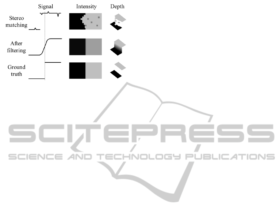
Figure 1: Effect of depth map reﬁnement.

an additional CCD sensor is required. In addition

depth map-image registration is required because sen-

sors’ positions are different. However,the registration

tends to be violated at object boundaries.

In the real-time stereo matching and the depth sen-

sor acquisition, both methods require noise reduction,

object boundaries recovering are required. Therefore,

to correct the depth at object boundary, and to remove

noise on depth maps, we propose a reﬁnement ﬁlter

for depth maps from stereo image pair or depth sen-

sors. For real-time applications, we keep the compu-

tational cost of the ﬁlter low.

The rest of this paper is organized as follows.

Sec. 2 describes related works of reﬁnement ﬁlters.

Proposed methods are presented in Sec. 3, and exper-

imental results are shown in Sec. 4. Sec. 5 concludes

this paper.

2 RELATED WORKS

Recently, depth map reﬁnement ﬁlters are focused.

Requirements for the reﬁnement ﬁlter are; capability

of edge correction, noise reduction, and edge keeping.

Figure 1 shows the effect of depth map reﬁnement.

Input depth signals are noisy and edge at boundary

is not correct. After reﬁnement ﬁlter, noise on depth

signal is removed and depth at boundary is corrected.

However unwanted slope blur at the boundary occurs.

The slope means that object boundary is smoothly

connected, but this is a fake signal. Thus keeping the

blur size small or removing the blur is important for

the reﬁnement.

The depth map reﬁnement ﬁlters are often edge-

preserving ﬁlter, e.g. median ﬁlter. Bilateral ﬁl-

ter (Tomasi and Manduchi, 1998) is an early approach

of them. The bilateral ﬁlter can remove noise while

preserving edges, but the performance of edge keep-

ing and noise reduction is trade-off. When the im-

age has large noises, the performance of edge keep-

ing becomes low to remove the noises. In addi-

tion, only Gaussian noise can be removed by the ﬁl-

ter, although depth map contains spike, speckle/blob

and non-Gaussian noises. Moreover, the inaccuracy

around object boundaries cannot be correct well.

Now, a variant called joint bilateral ﬁlter (or cross

bilateral ﬁlter) (Pestschnigg et al., 2004; Eisemann

and Durand, 2004; Kopf et al., 2007) relaxes bilat-

eral ﬁlter’s problem well by adding additional infor-

mation. The information is an original RGB im-

age used in depth estimation. This method regards

the depth map as a ﬁltering target, and the original

RGB image as a kernel computation target. The ﬁl-

ter makes the kernel by color or intensity values of

the RGB image instead of depth values. The ﬁlter

can smooth small non-Gaussian noises. In addition

the ﬁlter can ﬁt edges in the depth map around an

object to edges in the natural image’s object. How-

ever, the joint depth and image processing make a

new problem. The joint bilateral ﬁlter spreads blur-

ring to the outside of the depth map due to mixed

pixels, and outliers. Mixed pixels in natural images

occur on foreground and background boundaries and

they are caused by CCD sensor’s aliasing and optical

lens blur. The joint bilateral ﬁlter transfers the blur

to the depth map. In addition, impulse outliers and

large size noises on the depth map are diffused by the

ﬁltering.

Some methods can reduce this type of the blur

in some degree. Multilateral ﬁlter (Lai et al., 2010)

has three weights which are space, color and addi-

tional depth weight. The depth weight wants to keep

the shape of the edge of the depth map so that the

weight suspends blurring. Unfortunately, the weight

also loses an ability of the object boundary recover-

ing.

Cost volume based reﬁnement ﬁlter (Yang et al.,

2007) and its speedup approximation (Yang et al.,

2010) have better performance. The methods can cor-

rect depth edge and can remove spike noise and small

size speckle noise without diffusion. In addition the

method hardly generates blur at object boundaries. In

the processing of the cost volume ﬁlter, cost slices

which indicate every possibility of a depth value at

each pixel is computed, and all slices of each depth

level are stacked. The set of stacked slices are called

cost volume. Then, each slice is ﬁltered by the joint

bilateral ﬁlter slice by slice at each depth level. The

possibility is computed by a difference between an

initial depth and each depth level values. The method

performs d (depth search range) times bilateral ﬁlters,

and also iterates the multiple bilateral ﬁltering pro-

cess. Thus the method consumes a lot of time.

The reﬁnement ﬁlter which meets all requirements

WeightedJointBilateralFilterwithSlopeDepthCompensationFilterforDepthMapRefinement

301

is only cost volume reﬁnement, but it is cost consum-

ing. Thus a fast ﬁlter which meets all requirements is

an open question. Therefore, we present a new reﬁne-

ment ﬁlter to remove impulse/speckle noises, recover

object shapes and suppress the blurs with low com-

putational cost. The reﬁnement contains two ﬁlters;

one is weighted joint bilateral ﬁlter which is a variant

of joint bilateral ﬁlter and can reduce the boundary’s

blurs size, and the other is the slope depth compensa-

tion ﬁlter which eliminates depth slopes or blurs be-

tween a foreground and background objects.

3 PROPOSED FILTER

3.1 Weighted Joint Bilateral Filter

Our ﬁlter can reduce noises and correct object bound-

aries without large blur by using an input natural im-

age and a depth map. The ﬁlter is a variant of the joint

bilateral ﬁlter, and we call the ﬁlter weighted joint bi-

lateral ﬁlter (WJBF).

We add a weight factor to the joint bilateral ﬁlter.

The ﬁlter is deﬁned by the following formula:

∑

s∈N

w(p

p, s

s)c(I

, I

∑

s∈N

w(p

p, s

s)c(I

, I

, (1)

w(x

x, y

y) = e

−

(

||x

x−y

y||

)

, c(x

x, y

y) = e

−

(

||x

x−y

y||

)

where p

p = coordinate of current pixel, s

s = coordinate

of support pixel centered around pixel p

p, I = input nat-

ural image, D = input/output depth map, N = aggre-

gating set of support pixel s

s, w = spatial kernel weight

function, c = color/range kernel weight function, and

each weight function is Gaussian distribution (σ

, σ

const.). || · ||

is L2 norm function, and R

= weight

map. This ﬁlter is an equivalent joint bilateral ﬁlter

except for the weight map R. If the weight map is

uniform, for example all values of the weighted map

are set to 1, the weighted joint bilateral ﬁlter becomes

the joint bilateral ﬁlter.

The Eq. (1) is separated into 2 parts; one is a ker-

nel weighting part and the other is a weighting of val-

ues of ﬁltering target part. The former is w and c, and

the latter is R. The value’s weight R controls amount

of inﬂuence of depth value on a pixel and is ﬁxed over

the image ﬁltering. Thus we should set high weight at

a pixel which has a reliable depth value.

We want to set the joint bilateral kernel weight of

support pixels on another object to no weight. In the

joint bilateral ﬁlter case, the kernel weight between a

current pixel locates on an object boundary and sup-

port pixel on another object tend to have medium ker-

nel weight due to a mixed pixel on the object bound-

ary.

(a) Input natural image (b) Input depth map

Figure 2: Example of weight map.

The unwanted weight causes blurs on the depth

map near the object boundary. The depth values

around the object discontinuities are unreliable, so we

should set the weight of the depth value R to low.

In addition, impulse outliers or outliers in speck-

les/blobs are unreliable. Small speckles may be miss

estimated regions. The region should be set to no

weight. Figure 2(b) shows an example of impulse or

speckles/blobs in a depth map. If we cannot ignore

these regions, the regionsof speckle noise are diffused

by a smoothing ﬁlter. Basically, the object bound-

ary and the speckle region adversely affect depth map

reﬁnement. Thus we make a weight value for every

pixel, which is a weight map R, in advance to softly

ignore the ambiguous regions of the object boundary

and the speckle region.

In the weight map computation process, we clas-

sify pixels into located around object boundaries or

not, and speckle noise or not pixels. The result of

the soft classiﬁcation is represented by weighting val-

ues. In the classiﬁcation process, we have two as-

sumptions: First, if there is no boundary between the

current pixel and the support pixel, both pixels are

located at the same object. In this case, the depth

value and the intensity/color of the current pixel are

similar to these of the support pixels. Second, if

size of a connected component is small, the region

is speckle noised. In the connected component, dif-

ference among depth values is low.

Under the assumptions, the weight value R at s

s is:

∑

s∈N

′

· w(s

s, q

q)c(I

, I

−

(

||D

−D

)

, (2)

where q

q = coordinate of support pixel centered around

pixel s

s, N

′

= aggregating set of support pixel q

VISAPP2013-InternationalConferenceonComputerVisionTheoryandApplications

302

w(s

s, q

q) and c(I

, I

) are same functions as (1). How-

ever, equation (2) has an additional term of the dif-

ference of the depth values between the current and

the support pixel. M

is a speckle region mask. The

speckle mask has two weight values which is 0 and 1.

The areas of weight value 0 are the speckle regions,

and the areas of weight value 1 are non-speckle re-

gions.

The ﬁrst assumption is calculated by distance

of the intensity and the depth value of between

the current pixel and the support pixels. The sec-

ond assumption of the speckle regions is represented

by the speckle mask. This mask is made by the

initial depth map using the speckle detection ﬁl-

ter. The speckle detection ﬁlter has two parameters.

They are upper threshold of speckle component size

(speckleWindowSize) and allowable difference range

in the speckle (speckleRange). The speckle detection

ﬁlter judges region to be a speckle by whether or not

the region size is smaller than the speckle window

size and the region value is larger than the speckle

range. If some areas judged the speckle regions by

the speckle detection ﬁlter in the initial depth map,

the weight of the speckle region is set to 0.

Figure 2 shows examples of an input image, a

noisy depth map, a speckle mask and a weight map. If

regions are speckled pixels, the speckle regions have

no weight. If not, all value of M

is set to 1, so the

weight map has some weight values. As a result,

boundary regions in the images and the depth map

have small weight. We can softly ignore boundary’s

depth values and speckle’s depth values, therefore,

the weighted bilateral ﬁlter with the weight map can

suppress boundary blur, can correct image boundary

well, and can reduce the speckle noises.

In the brute force computation of the ﬁltering a

pixel has the fourfold loops (vertical and horizon-

tal ﬁltering kernel and vertical and horizontal weight

map kernel loops), but the weight map is constant in

Eq. (1). Thus we compute the weight map before the

weighted joint bilateral ﬁltering for effective compu-

tation.

3.2 Slope Depth Compensation Filter

The weighted joint bilateral ﬁlter reﬁnes accuracy

around boundaries and smoothness on ﬂat regions,

but subtle blurs still remain in such cases, e.g. dif-

ference between foreground and background color

is small, and/or difference between foreground and

background depth value is large. The depth values

around the boundary are usually almost binary (fore-

ground/background); thus averaged depth values are

not suitable. The blurs make slopes between the fore-

(a) Tsukuba (b) Venus

Figure 3: Middlebury’s data sets.

ground and background depths. They do not exist

in the real environment. Consequently, these slopes

should be removed. We propose a new ﬁlter called

Slope depth compensation ﬁlter (SDCF).

The ﬁlter is deﬁned by the following formula:

SDCF

= D

INIT IAL

(3)

s.t. v

v = argmin

s∈W

||D

WJBF

− D

INITIAL

where D

is the depth map estimated by a method

X ∈ {INITIAL, WJBF, SDCF} , W is the aggregation

set of a support pixel, | · |

means L2 norm function,

p is target pixel position, s

s is support pixel position,

and v

v is a pixel position which points the minimum of

the function.

This ﬁlter replaces the values blurred by the

weighted joint bilateral ﬁlter as the nearest values

in the support region on the no ﬁltered version of

INIT IAL

. There are not mixed values in no ﬁltered

version so that the ﬁlter completely removes blended

values.

At ﬁrst, the depth map D

INIT IAL

is obtained by a

stereo matching method, and then the depth map is

ﬁltered by the weighted joint bilateral ﬁlter (output is

written as D

WJBF

), and ﬁnally the depth map is com-

pensated by depth slope compensation ﬁlter (D

DSCF

4 EXPERIMENTAL RESULTS

4.1 Experimental Setups

We evaluate the weighted joint bilateral ﬁlter (WJBF)

with the slope depth compensation ﬁlter (SDCF). The

WeightedJointBilateralFilterwithSlopeDepthCompensationFilterforDepthMapRefinement

303

Table 1: Error Rate (%) of depth maps: Results of various stereo matching methods (block matching (BM), dynamic program-

ming (DP), semi-global block matching (SGBM), efﬁcient large scale stereo (ELAS), and double belief propagation (DBP))

with proposed ﬁlter or reﬁnement ﬁlters (median ﬁlter (MF), bilateral ﬁlter (BF), joint bilateral ﬁlter (JBF), multi lateral ﬁlter

(MLF), and ﬁlter in constant space belief propagation (CSBP)).

Tsukuba Venus Teddy Cones

nonocc all disc nonocc all disc nonocc all disc nonocc all disc

BMh 10.78 12.22 20.03 12.58 13.79 23.06 16.17 24.25 29.89 7.76 17.19 20.01

BMh & WJBF

3.39 4.21 13.95 1.69 2.60 13.66 12.18 20.63 24.04 3.94 12.38 11.78

BMh & Proposed 3.25 4.04 13.15 1.36 2.07 9.51 9.20 17.55 20.20 3.03 11.38 9.04

BMm 7.50 8.75 18.84 5.01 5.96 16.49 12.36 18.10 24.94 5.56 11.54 15.47

BMm & WJBF 3.14 3.78 14.59 2.62 3.17 8.52 10.09 15.84 21.84 4.57 10.43 13.67

BMm & Proposed

2.89 3.45 13.29 1.49 1.94 4.22 8.79 14.24 19.22 3.13 8.53 9.21

BMl 4.60 5.93 17.99 2.08 2.91 16.11 10.63 15.51 26.43 4.97 10.46 14.31

BMl & WJBF 2.69 3.20 12.57 1.51 2.14 9.55 9.41 14.41 22.56 4.61 10.08 13.52

BMl & Proposed

2.54 3.25 11.53 1.03 1.50 5.11 8.90 13.71 21.05 3.25 8.43 9.62

DP 4.12 5.04 11.95 10.10 11.03 21.03 14.00 21.58 20.56 10.54 19.10 21.10

DP & WJBF

2.63 3.40 11.12 6.77 7.17 20.65 9.81 17.12 18.44 7.98 15.92 18.49

DP & Proposed 2.49 3.22 10.74 6.01 6.36 18.12 9.22 16.53 16.98 7.12 15.64 16.05

SGBM 3.98 5.56 15.47 1.33 2.59 15.23 7.60 14.83 20.90 4.55 11.33 12.81

SGBM & WJBF

2.42 3.09 9.83 0.46 0.97 5.02 6.33 13.41 17.53 3.89 10.22 11.58

SGBM & Proposed 2.34 2.59 9.42 0.36 0.83 3.73 5.68 12.43 15.42 2.58 8.62 7.68

ELAS 3.99 5.45 18.14 1.84 2.55 20.28 7.99 14.69 22.33 6.85 14.55 17.30

ELAS & WJBF 2.96 3.68 13.33 0.71 1.18 7.82 6.55 13.23 17.60 5.35 12.80 13.90

ELAS & Proposed

2.87 3.54 12.86 0.55 0.81 5.65 6.07 12.48 15.67 4.58 12.04 11.69

DBP 0.88 1.29 4.76 0.13 0.45 1.87 3.53 8.30 9.63 2.90 8.78 7.79

DBP & WJBF 0.88 1.31 4.78 0.15 0.39 2.04 3.57 8.37 9.80 2.97 8.74 8.05

DBP & Proposed

0.83 1.19 4.78 0.10 0.32 1.44 3.56 8.31 9.69 2.87 8.62 7.74

BMl & MF 3.54 4.72 16.96 1.50 2.32 16.12 10.35 15.41 25.96 4.52 9.99 13.16

BMl & BF

3.92 5.29 16.73 1.77 2.63 16.90 10.51 15.42 26.21 4.76 10.24 13.91

BMl & JBF 4.57 5.82 19.37 2.14 2.98 16.64 11.50 17.17 29.37 6.77 12.37 19.59

BMl & MLF

4.25 5.34 18.02 2.73 3.74 26.08 11.45 17.15 29.17 6.54 12.04 18.93

BMl & CSBP 4.79 6.56 17.68 2.42 3.40 21.17 11.31 16.08 28.81 5.49 11.31 15.55

combination of WJBF and the SDCF is called pro-

posed method (in short Proposed). In our experi-

ments, we evaluate accuracy improvement of the pro-

posed ﬁlter for various types of depth map. In ad-

dition, we reveal advantage of its computational cost.

Moreover we show an example of reﬁnement of depth

map from Microsoft Kinect.

We use the Middlebury’s data sets (Scharstein and

Szeliski, 2002) are used for our stereo evaluation

in the experiments. Data sets are Tsukuba, Venus,

Teddy and Cones (Fig. 3). The image resolution

and depth search range of each image are Tsukuba

(384 × 288, 16), Venus (434 × 383, 32), Teddy and

Cones (450× 375, 64), respectively.

We evaluate the proposed reﬁnement ﬁlter for var-

ious depth inputs. Stereo matching methods for the

input depth maps are block matching (BM), dynamic

programming (DP) (Ohta and Kanade, 1985), semi-

global block matching (SGBM) (Hirschmuller, 2008),

efﬁcient large-scale stereo (ELAS) (Geiger et al.,

2010) and double belief propagation (DBP) (Yang

et al., 2008).

We prepared three patterns of the BM’s depth

map according to the amount of noises. They are

high (BMh), middle (BMm) and low noise depth maps

Table 2: Comparing proposed method with cost volume re-

ﬁnement (Teddy).

nonocc all disc

BMh 16.17 24.25 29.89

BMh & CVR 8.15 16.25 20.49

BMh & Proposed 9.20 17.55 20.20

BMl 10.63 15.51 26.43

BMl & CVR 8.98 13.58 21.58

BMl & Proposed 8.90 13.71 21.05

SGBM 7.60 14.83 20.90

SGBM & CVR 5.93 12.93 16.39

SGBM & Proposed 5.68 12.43 15.42

(BMl) (See Figs. 6(a), 6(d), 6(g)). The characteris-

tics of the other depth maps are as follows. The DP,

SGBM and ELAS are computed by stereo method

which has near real-time performance, whose depth

maps are middle accuracy (See Figs. 7(a), 8(a), 9(a)).

The DBP (10(a))) is the most accurate method but it

takes much time (several minutes).

In addition, the effect of the proposed reﬁne-

ment ﬁlter is veriﬁed by following competitive re-

ﬁnement ﬁlters. These are the low noise BM’s

depth map with median ﬁlter (MF), bilateral ﬁlter

(BF) (Tomasi and Manduchi, 1998), joint bilateral

ﬁlter (JBF) (Pestschnigg et al., 2004; Eisemann and

VISAPP2013-InternationalConferenceonComputerVisionTheoryandApplications

304

Durand, 2004; Kopf et al., 2007), multilateral ﬁlter

(MLF) (Lai et al., 2010) and speedup version of (Yang

et al., 2007) used in constant space belief propagation

(CSBP) (Yang et al., 2010) are used as reﬁnement ﬁl-

ters. Furthermore, we compare our proposed method

with a cost volume reﬁnement method (Yang et al.,

2007). In the cost volume reﬁnement, we use joint bi-

lateral ﬁlter for cost slice ﬁltering, and we use inputs

depth maps with BMh, BMl and SGBM.

4.2 Results

The resulting depth maps are shown in Fig. 6 to

Fig. 11 (only Teddy’s results are shown due to the

room of the space at the end of the paper). There

are ﬁve parameters at weighted image generation

and two parameters at ﬁltering. The parameters

of proposed method at weighted image generation

are (σ

, σ

, speckleWindowSize, speckleRange) =

(15.4, 5.1, 1.4, 38, 1), and those at ﬁltering are

(σ

, σ

) = (15.3, 10.7) using BMh depth map. There

parameters are experimentally determined in all

cases. The results of error rate are shown in Tab. 1.

We use the error rate deﬁned in (Scharstein and

Szeliski, 2002). It is calculated by a percentage of the

error pixel of input depth map. Difference between

the input depth map and the ground truth depth map

in the error pixel has over a threshold value (set to 1

in these experiments). In Tab. 1 and Tab. 2, “nonocc”,

“all” and “disc” locate different region, respectively.

The header row “nonocc” evaluates in non-occluded

regions. The header row “all” evaluates in all regions.

The header row “disc” evaluates in regions near depth

discontinuities.

In Table 1, our proposed method can improve

accuracy in all competitive stereo matching meth-

ods and in any data sets, except for DBP. Especially,

amount of the improvement is bigger when accuracy

of depth maps is low. Such roughly estimated depth

maps contain a lot of region of estimation error and

obscure edges. Thus, the proposed method works

well for these depth maps because of noise reduction

and correcting object boundary ability. But, as for

an accurate depth map, such as DBP, the proposed

method has almost no effect. This is because that

there is no region which is possible to be improved.

Instead, in some cases, the error rate is increasing ac-

cording to generated invalid depth value by mixing

some depth values.

Moreover, Table 1 shows that the effect of using

only WJBF and using the proposed method (WJBF

+ SDCF). The effect of the WJBF becomes higher

when the accuracy of input depth map is low. This

is because that the WJBF removes the whole noise,

+Filter

SGBM

ELAS

Image size (n x n) [pixel]

6000

5000

4000

3000

2000

1000

Time [ms]

128 384 640 896 1152 1408 1664 1920

(a) Y axis is until 6000 ms

+Filter

SGBM

ELAS

Time [ms]

Image size (n x n) [pixel]

128 384 640 896 1152 1408 1664 1920

100

200

300

400

(b) Y axis is until 400ms

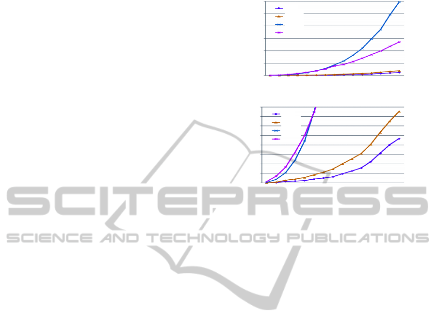
Figure 4: Computational time of each method.

but the SDCF compensate only blurred edge. Thus,

these methods differ in the effect range greatly.

In addition, our proposed reﬁnement ﬁlter has the

best performance among all competitive reﬁnement

ﬁlters (cost volume reﬁnement is discussed later).

This is because that the MF and the BF can reduce

noise, but, cannot correct object edges. The JBF and

the MLF can reduce noise and correct object edges,

but cannot correct all blur on edges according to mix-

ing some depth values. On the other hands, proposed

method can reduce noise, correct object edges and

control edge blurring.

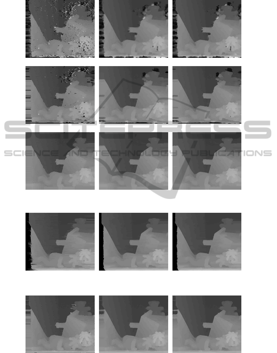
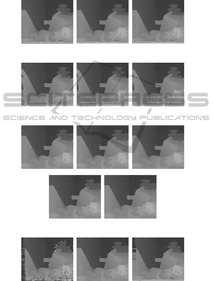
Here, the effect of the proposed method is consid-

ered from Fig. 6 to Fig. 10. In Fig. 6, depth maps

of (a), (d) and (g) is input depth map with BM. Each

depth map is low accuracy which has many noise and

incorrect object edges. Depth maps of (b), (e) and (h)

are reﬁned by WJBF. These depth maps are reduced

noise and corrected object edges through the WJBF.

But, blur edges occur in object boundary. Whereat us-

ing SDCF, the blur of boundary edges is compensated

in depth maps of (c), (f) and (i). The same effect is

shown by Fig. 7 to Fig. 9. In Fig. 7(a), the effect of

noise reduction is shown. A noise of estimation error

using the DP is reduced by the WJBF. Also, the effect

of edge correction is shown in Fig. 8 and Fig. 9. An

irregularity of boundary edges is corrected by SDCF.

On the other hands, the effect of our proposed method

is not shown in Fig. 10(a). A depth map of (a) using

DBP has almost no noise and correct edges. Thus, our

proposed method hardly makes an effect.

Here, we consider our proposed method and the

WeightedJointBilateralFilterwithSlopeDepthCompensationFilterforDepthMapRefinement

305

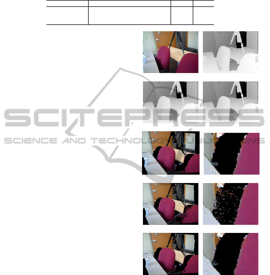
Table 3: Comparing running time (ms) of BM plus proposed ﬁlter with selected stereo methods. Kernel size is 7× 7.

Data Set BM Proposed BM+Proposed SGBM ELAS

tsukuba 5.7 4.1 9.8 28.8 61.1

venus 8.4 6.1 14.5 45.9 110.0

teddy and cones 10.5 7.4 17.9 71.4 168.2

cost volume reﬁnement method (CVR). Table 2 and

Fig. 12 show performance of CVR. The input depth

maps are BMh, BMl and SGBM and we use Teddy

data set (Other data sets have the almost same ten-

dency). Comparing the CVR with the proposed

method with each depth map inputs, the performance

of the proposed method is the same or better than

CVR with BMl and SGBM. In the highest noise case,

CVR has the better performance than the proposed

ﬁlter. Thus CVR has strong noise reduction perfor-

mance but reduce some detail.

The notable factor of CVR is computational cost.

The cost volume is calculated by stacking the cost

slice of the each depth value which is difference be-

tween an input depth and each depth values, and,

ﬁlters every stack. Thus, this method is expensive.

For example, 64 times bilateral ﬁltering is required in

Teddy case, and about 32 times slower than the pro-

posed method. Our proposed method has real-time

capability. Therefore, if the accuracy of an acquired

depth maps is comparable, our proposed method is

more effective than CVR.

Table 3 and Fig. 4 show the result of the running

time with Intel Core i7-920 2.93GHz. Here, compet-

itive methods are SGBM and ELAS which are near

real-time methods in optimized methods. The BM

with the proposed method is faster than the SGBM

and the ELAS for any data set. In addition, reﬁnement

ﬁlters depend only on the image resolution, while op-

timization processes (e.g. SGBM) depend also on the

depth search range; thus the gap of the running time

between the proposed method and optimized method

like the SGBM more increase as the image resolu-

tion and the search range become larger. Recently,

image and display resolution are rapidly improved,

thus the proposed method is favorable. Figure 4

shows computational time of various size of simu-

late image data. The lowest size of the input image

is 128 × 128 and its search range is 8. The input im-

ages are generated by multiplying the minimum size

image, such as (256 × 256, 16), (384 × 384, 24), ...,

(1920×1920, 120). The results show that BM is quite

faster than the SGBM and ELAS, and the computa-

tional cost of the proposed reﬁnement ﬁlter is quite

low.

We can also use the proposed ﬁlter for depth maps

from Microsoft Kinect. Figure 5 shows experimental

results of a depth map from Kinect depth sensor, and

(a) Kinect image (b) Kinect’s depth

(e) rendering using (b) (f) zoomed image (e)

(g) rendering using (c) (h) zoomed image (g)

(i) rendering using (d) (j) zoomed image (i)

Figure 5: Results of reﬁned depth map and warped view

from Kinect depth map.

the sequence is uploaded by (Lai et al., 2011). In this

experiment, we reﬁne the depth map from the Kinect

depth sensor and synthesis a free viewpoint image.

The free viewpoint image synthesis is performed

by the depth image based rendering (Mori et al.,

2009). The non-ﬁltered depth map of getting the

Kinect has rough edges (Fig. 5(b)). Thus, the edge

of a composite image which uses non ﬁltered depth

map is defectiveness (See the chair region of Fig. 5(e,

VISAPP2013-InternationalConferenceonComputerVisionTheoryandApplications

306

(a) BMh (b) BMh & WJBF (c) BMh & Proposed

(d) BMm (e) BMm & WJBF (f) BMm & Proposed

(g) BMl (h) BMl & WJBF (i) BMl & Proposed

Figure 6: Results: block matching.

(a) DP (b) DP & WJBF (c) DP & Proposed

Figure 7: Results: dynamic programming.

(a) SGBM (b) SGBM & WJBF (c) SGBM & Proposed

Figure 8: Results: semi-global block matching.

WeightedJointBilateralFilterwithSlopeDepthCompensationFilterforDepthMapRefinement

307

(a) ELAS (b) ELAS & WJBF (c) ELAS & Proposed

Figure 9: Results: efﬁcient large-scale.

(a) DBP (b) DBP & WJBF (c) DBP & Proposed

Figure 10: Results: double belief propagation.

(a) MF (b) BF (c) JBF

(d) MLF (e) CSBP

Figure 11: Results: competitive reﬁnement ﬁlters.

(a) BMh & CVR (b) BMl & CVR (c) SGBM & CVR

Figure 12: Results: cost volume reﬁnement.

VISAPP2013-InternationalConferenceonComputerVisionTheoryandApplications

308

f)). The depth ﬁltered by joint bilateral ﬁlter has

blurs around the boundary (Fig. 5(c)), the render-

ing images are scattered around the object boundary

(Fig. 5(g, h)). In contrast, the depth map ﬁltered by

the proposed ﬁlter has corrected edges and no blurs

(Fig. 5(d)). As a result, the edge of the composite

image (Fig. 5(i), (j)) is more corrective then the non-

ﬁltered or joint bilateral ﬁltered it.

5 CONCLUSIONS

In this paper, we proposed a reﬁnement ﬁlter set for

depth map improvement—called weight joint bilat-

eral ﬁlter and slope depth compensation ﬁlter. The

proposed method can reduce depth noise and correct

object boundary edge without boundary blurring, and

it has real-time performance. Experimental results

showed that our proposed ﬁlter can improve accuracy

of depth maps from various stereo matching methods,

and has the best performance among the compara-

tive reﬁnement ﬁlters. Especially, amount of improve-

ment is large when an input depth map is not accurate.

In such case, computational time of a stereo matching

method is low. Exception case is using fairly opti-

mized depth map, such as double belief propagation.

However the method takes a lot of time. In addi-

tion, its computational speed is faster than the fastest

Markov random ﬁeld optimization algorithm of semi-

global block matching. Moreover, the ﬁlter can apply

the depth map from Kinect, and then the quality of the

synthesized image is up.

In our future work, we will investigate dependen-

cies of input natural images and depth maps, and ver-

ify the proposed ﬁlter’s parameters.

ACKNOWLEDGEMENTS

The authors thank Prof. Shinji Sugawara for valu-

able discussions. This work was partly supported

by the Grand-In-Aid for Young Scientists (B) of

Japan Society for the Promotion of Science under

Grant 22700174, and SCOPE (Strategic Information

and Communications R&D Promotion Programme)

122106001 of the Ministry of Internal Affairs and

Communications of Japan.

REFERENCES

Boykov, Y., Veksler, O., and Zabih, R. (2001). Fast approxi-

mate energy minimization via graph cuts. IEEE Trans.

PAMI, 23(11):1222–1239.

Eisemann, E. and Durand, F. (2004). Flash photography

enhancement via intrinsic relighting. ACM Trans. on

Graphics, 23(3):673–678.

Fukushima, N., Fujii, T., Ishibashi, Y., Yendo, T., and Tan-

imoto, M. (2010). Real-time free viewpoint image

rendering by using fast multi-pass dynamic program-

ming. In 3DTV-Conference: The True Vision-Capture,

Transmission and Display of 3D Video (3DTV-CON),

pages 1–4.

Fukushima, N. and Ishibashi, Y. (2011). Client driven sys-

tem of depth image based rendering. ECTI Trans. CIT,

5(2):15–23.

Geiger, A., Roser, M., and Urtasun, R. (2010). Efﬁcient

large-scale stereo matching. In Asian Conference of

Computer Vision, volume 6492, pages 25–38.

Hirschmuller, H. (2008). Stereo processing by semiglobal

matching and mutual information. IEEE Trans. PAMI,

30(2):328 –341.

Kopf, J., Lischinski, M. F. C. D., and Uyttendaele, M.

(2007). Joint bilateral upsampling. ACM Trans. on

Graphics, 26(3):96.

Lai, K., Bo, L., Ren, X., and Fox, D. (2011). A large-scale

hierarchical multi-view rgb-d object dataset. In IEEE

International Conference on Robotics and Automation

(ICRA), pages 1817–1824.

Lai, P. L., Tian, D., and Lopez, P. (2010). Depth map pro-

cessing with iterative joint multilateral ﬁltering. In

Picture Coding Symposium, pages 9–12.

Mori, Y., Fukushima, N., Yendo, T., Fujii, T., and Tanimoto,

M. (2009). View generation 3d warping using depth

information for ftv. Signal Processing: Image Com-

munication, 24(1–2):65–72.

Ohta, Y. and Kanade, T. (1985). Stereo by intra - and inter-

scanline search using dynamic programming. IEEE

Trans. PAMI, 7(2):139–154.

Pestschnigg, G., Szeliski, R., Agrawala, M., Cohen, M.,

Hoppe, H., and Toyama, K. (2004). Digital photogra-

phy with ﬂash and no-ﬂash image pairs. ACM Trans.

on Graphics, 23(3):664–672.

Scharstein, D. and Szeliski, R. (2002). A taxonomy and

evaluation of depth two-frame stereo correspondence

algorithms. International Journal of Computer Vision,

47(1):7–42.

Sun, J., Zheng, N. N., and Shum, H. Y. (2003). Stereo

matching using belief propagation. IEEE Trans.

PAMI, 25(7):787–800.

Tomasi, C. and Manduchi, R. (1998). Bilateral ﬁltering for

gray and color image. In International Conference of

Computer Vision, pages 839–846.

Wildeboer, M. O., Fukushima, N., Yendo, T., Tehrani, M. P.,

Fujii, T., and Tanimoto, M. (2010). A semi-automatic

multi-view depth estimation method. In Proceedings

of SPIE Visual Communications and Image Process-

ing 2010, volume 7744.

Yang, Q., Wang, L., and Ahuja, N. (2010). A constant-

space belief propagation algorithm for stereo match-

ing. In Computer Vision and Pattern Recognition,

pages 1458–1465.

Yang, Q., Wang, L., Yang, R., Stewenius, H., and Nister,

D. (2008). Stereo matching with color-weighted cor-

relation, hierarchial belief propagation and occlusion

handling. IEEE Trans. PAMI.

Yang, Q., Yang, R., Davis, J., and Nister, D. (2007). Spatial-

depth super resolution for range images. In Computer

Vision and Pattern Recognition, pages 1–8.

WeightedJointBilateralFilterwithSlopeDepthCompensationFilterforDepthMapRefinement

309