
Planar Motion and Hand-eye Calibration using Inter-image
Homographies from a Planar Scene
M
˚
arten Wadenb
¨
ack and Anders Heyden
Centre for Mathematical Sciences, Lund University, Lund, Sweden
Keywords:
Visual Navigation, Planar Motion, SLAM, Homography, Tilted Camera.
Abstract:
In this paper we consider a mobile platform performing partial hand-eye calibration and Simultaneous Loc-
alisation and Mapping (SLAM) using images of the floor along with the assumptions of planar motion and
constant internal camera parameters. The method used is based on a direct parametrisation of the camera
motion, combined with an iterative scheme for determining the motion parameters from inter-image homo-
graphies. Experiments are carried out on both real and synthetic data. For the real data, the estimates obtained
are compared to measurements by an industrial robot, which serve as ground truth. The results demonstrate
that our method produces consistent estimates of the camera position and orientation. We also make some
remarks about patterns of motion for which the method fails.
1 INTRODUCTION
The development of algorithms for Simultaneous
Localisation and Mapping (SLAM) has been a ma-
jor focus in robotics research the past few decades.
Such algorithms aim at enabling a mobile platform to
explore and map its surroundings, while at the same
time maintaining accurate knowledge of its position.
Many types of sensors may be used to this end, and
are often combined to supplement each other.
For the mapping part of SLAM, a reconstruction
(broadly interpreted) must be created from the scene.
For some work on SLAM using visual sensors, see
for example (Davison, 2003), (Karlsson et al., 2005)
and (Koch et al., 2010). Scene reconstruction from
images is a well studied problem in computer vision,
and is still a very active research area. Since the intro-
duction of the fundamental matrix in (Faugeras, 1992)
and (Hartley, 1992), epipolar geometry has been the
foundation of many successful approaches to visual
reconstruction.
However, a planar or near-planar scene is well
known to be a degenerate or ill-conditioned case for
reconstruction based on the fundamental matrix and
similar approaches. Since planar scenes and objects
are very common in man-made or indoor environ-
ments, a navigation system intended to operate in
such environments must take care to avoid degener-
acy. Planar homographies, on the other hand, are par-
ticularly well suited to planar scenes, but are unable to
describe general 3D structure. This insight has been
utilised for visual navigation in (Liang and Pears,
2002) and (Hajjdiab and Lagani
`
ere, 2004), among
others.
In this paper we shall consider a single camera,
with square pixels and zero skew, moving at a con-
stant height above the floor. We will further assume
that the internal parameters of the camera are con-
stant, and that the camera orientation is fixed except
for a rotation about the normal to the floor plane. Us-
ing inter-image homographies not only avoids the de-
generacy issue mentioned above, but in addition al-
lows us to use an explicit parametrisation of this par-
ticular kind of camera motion.
In the case where the inter-image homographies
describe a Euclidean (or, in general, an affine) trans-
formation, the motion parameters are easily recovered
using the QR decomposition. This happens when the
image plane is parallel to the floor. In the presence of
a tilt, however, it is not as straightforward to extract
the motion information from the homographies. The
main contribution of this paper is a method to com-
pute both the tilt and the motion information from a
single homography.
Another reason for estimating the tilt is that only
rectified images may be stitched consistently into a
mosaic. A visual navigation system based on a sparse
feature based map of the floor plane also needs recti-
fied images to construct the map. It is in general not
trivial to mount a camera with very high precision, so
164
Wadenbäck M. and Heyden A..
Planar Motion and Hand-eye Calibration using Inter-image Homographies from a Planar Scene.
DOI: 10.5220/0004293701640168
In Proceedings of the International Conference on Computer Vision Theory and Applications (VISAPP-2013), pages 164-168
ISBN: 978-989-8565-48-8
Copyright
c
2013 SCITEPRESS (Science and Technology Publications, Lda.)

avoiding the need for this would be useful.
Determining the tilt can also be seen as a partial
hand-eye calibration. The original formulation of the
hand-eye calibration problem was to recover the re-
lative orientation between a robot arm and a camera
mounted on the arm. Tsai and Lenz showed that with
known 3D feature points, known motion of the ro-
bot arm, and known transformations A and B, the un-
known relative orientation X can be determined from
the equation AX = XB (Tsai and Lenz, 1989). The
problem was later reformulated using quaternions to
parametrise rotations and 3 ×4 camera matrices in-
stead of classical transformation matrices (Horaud
and Dornaika, 1995).
2 CAMERA PARAMETRISATION
We assume that the camera is mounted rigidly onto a
mobile platform, and directed towards the floor. This
means that the position and orientation of the cam-
era can be parametrised by a translation vector t and
a rotation in the floor plane of an angle ϕ. The tilt
is described by the constant angles ψ and θ. Both
the translation and the three angles will be estimated.
The camera is assumed to move in the plane z = 0,
and the ground plane is taken to be at z = 1. This is
not a restriction, since it only reflects our choice of
the world coordinate system and global scale fixation
(corresponding to the unknown focal length).
We will consider two consecutive images, A and
B, with associated camera matrices
P
A
= R
ψθ
[I | 0],
P
B
= R
ψθ
R
ϕ
[I | −t].
(1)
Here R
ψθ
is a rotation of θ around the y-axis followed
by a rotation of ψ around the x-axis, and R
ϕ
is a rota-
tion of ϕ around the z-axis (the floor normal).
Using (1), one can easily verify that the homo-
graphy H from A to B is
H = λR
ψθ
R
ϕ
TR
T
ψθ
, (2)
for any non-zero λ ∈ R and with
T =
1 0 −t
x
0 1 −t
y
0 0 1
. (3)
3 TILT ESTIMATION
The presence of a tilt gives rise to perspective effects.
These distort the geometry perceived by the camera,
and prevent easy extraction of motion information. If
the tilt angles ψ and θ can be determined, one can
rectify the image and then use the QR decomposition
to retrieve the translation t and the free rotation ϕ.
To estimate ψ and θ, we derive equations that con-
tain these angles but which do not contain t and ϕ.
These equations will then be solved using an iterative
scheme.
3.1 Eliminating ϕ
Separating the tilt angles ψ and θ from the motion
parameters t and ϕ in (2), we get
R
T
ψθ
HR
ψθ
= λR
ϕ
T. (4)
Here, one notes that R
ϕ
can be eliminated by mul-
tiplying with the transpose from the left on both sides.
This results in the relation
R
T
ψθ
MR
ψθ
= λ
2
T
T
T, (5)
with (symmetric)
M =
m
11
m
12
m
13
m
12
m
22
m
23
m
13
m
23
m
33
= H
T
H. (6)
Since both sides of (5) are symmetric matrices,
one obtains six unique equations. Let L = R
T
ψθ
MR
ψθ
and R = λ
2
T
T
T be the left and right hand sides of
(5), respectively. Evaluating R , one obtains
R = λ
2
1 0 −t
x
0 1 −t
y
−t
x
−t
y
1+ t
2
x
+t
2
y
. (7)
3.2 Iterative Scheme
As described in Section 2, R
ψθ
= R
ψ
R
θ
is a rotation
of θ around the y-axis followed by a rotation of ψ
around the x-axis. Direct multiplication of the ro-
tation matrices allows us to evaluate L (though this
margin is too narrow to contain the result), and one
finds that L is a fourth degree expression in c
ψ
=
cosψ, s
ψ
= sinψ, c
θ
= cosθ and s
θ
= sinθ.
Noting that R
11
, R
12
and R
22
are independent of t,
the equations for ψ and θ become
L
11
−L
22
= 0
L
12
= 0
. (8)
But instead of trying to solve (8) for both ψ and θ at
the same time, we will iteratively alternate between
solving for one angle, with the other held fixed. This
reduces the problem of solving a fourth degree trigo-
nometric equation, so that we instead iterate and solve
a second degree equation in each iteration.
PlanarMotionandHand-eyeCalibrationusingInter-imageHomographiesfromaPlanarScene
165

Before explaining in detail how these equations
are solved, we first outline in Algorithm 1 the iterat-
ive scheme which produces an approximation to R
ψθ
.
Since
R
ψθ
= R
ψ
R
θ
=
c
θ
0 −s
θ
−s
ψ
s
θ
c
ψ
−s
ψ
c
θ
c
ψ
s
θ
s
ψ
c
ψ
c
θ
(9)
it is trivial to find ψ and θ from this approximation.
Algorithm 1: Iteratively approximate R
ψθ
. The steps on
line 6 and line 8 are detailed in Sections 3.2.1 and 3.2.2.
Since we “embed” into M the current approximation, we
may assume that the fixed angle is zero when solving for
the free one.
Input: An inter-image homography H
Output: An approximation R of R
ψθ
1:
b
M ← H
T
H
2: θ
0
← 0
3: R ← R
θ
0
4: for j = 1, ..., N do
5:
b
M ← R
T
θ
j−1
b
MR
θ
j−1
6: Solve for ψ
j
7:
b
M ← R
T
ψ
j
b
MR
ψ
j
8: Solve for θ
j
9: end for
10: R ← R
θ
0
R
ψ
1
R
θ
1
R
ψ
2
R
θ
2
···R
ψ
N
R
θ
N
3.2.1 Solving for ψ
Since c
ψ
and s
ψ
cannot both be zero, (8) is equivalent
to
L
11
−L
22
= 0
c
ψ
L
12
= 0
s
ψ
L
12
= 0
. (10)
By letting
b
M = R
T
θ
MR
θ
this can be written in matrix
form as
b
m
11
−
b
m
22
−2
b
m
23
b
m
11
−
b
m
33
b
m
12
b
m
13
0
0
b
m
12
b
m
13
c
2
ψ
c
ψ
s
ψ
s
2
ψ
= 0.
(11)
This means that (c
2
ψ
,c
ψ
s
ψ
,s
2
ψ
) lies in the null space of
the coefficient matrix in (11). For the moment
1
, let us
assume that we expect a one dimensional null space.
Due to measurement noise this will not be the case, so
instead we use the singular vector v = (v
1
,v
2
,v
3
) cor-
responding to the smallest singular value as our null
vector.
1
This is true for most patterns of motion. Section 4.2
demonstrates some specific patterns of motions for which
this is fragile.
Provided the singular vector v one obtains ψ as
ψ =
1
2
arcsin
2v
2
v
1
+ v
3
. (12)
3.2.2 Solving for θ
Now θ can be found in much a similar way as ψ.
Physical considerations imply that, at least for moder-
ately sized angles, R
ψ
R
θ
has approximately the same
effect on the camera as R
θ
R
ψ
. Examination of the
matrices confirms this for small angles.
Therefore, if
b
M = R
T
ψ
MR
ψ
, then
L
11
−L
22
= 0
c
θ
L
12
= 0
s
θ
L
12
= 0
, (13)
can be written in matrix form as
b
m
11
−
b
m
22
2
b
m
13
b
m
33
−
b
m
22
b
m
12
b
m
23
0
0
b
m
12
b
m
23
c
2
θ
c
θ
s
θ
s
2
θ
= 0. (14)
We find, in the same way as in Section 3.2.1 that
the null vector v can be used to find
θ =
1
2
arcsin
2v
2
v
1
+ v
3
. (15)
4 EXPERIMENTS
In order to test how well the tilt estimation works in
practice, fifty homographies of the form (2) were gen-
erated with random values for ψ, θ, ϕ and t. The true
angles and their corresponding estimates can be seen
in Figure 1.
4.1 Path Reconstruction
A simple path estimation has also been tried on both
synthetic and real data using the QR decomposition to
determine translation and planar rotation, after estim-
ating the tilt as described in Section 3. In the simu-
lation, noise of the magnitude corresponding to a few
pixels have been added to the points used to estim-
ate the homographies. Results for this experiment are
shown in Figure 2 and 3.
We have also carried out experiments with real
data. A camera mounted onto an industrial robot has
been used to take images, from which homograph-
ies were computed. The resulting reconstruction can
be seen in Figure 4. For comparison, we have ad-
ditionally estimated the non constant angle ϕ using
a method based on conjugate rotations, see (Liang
VISAPP2013-InternationalConferenceonComputerVisionTheoryandApplications
166
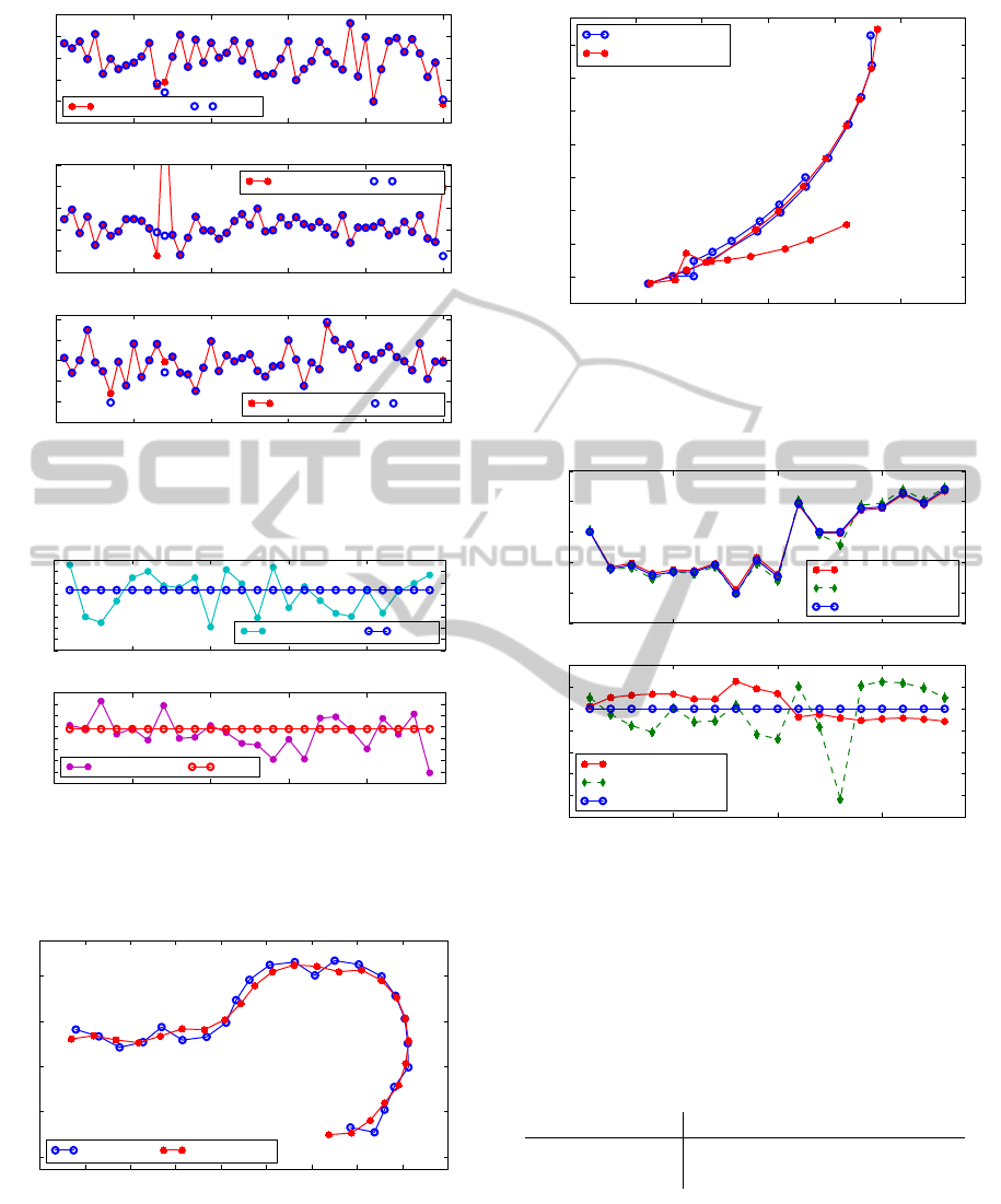
0 10 20 30 40 50
homography number
−15
−10
−5
0
5
10
θ (degrees)
estimated θ true θ
0 10 20 30 40 50
homography number
−20
−10
0
10
20
30
ψ (degrees)
estimated ψ true ψ
0 10 20 30 40 50
homography number
−150
−100
−50
0
50
100
ϕ (degrees)
estimated ϕ true ϕ
Figure 1: True and estimated values for ψ, θ and ϕ for fifty
randomly generated homographies. As can be seen, the es-
timation works well in most instances.
0 5 10 15 20 25
homography number
−4.0
−3.5
−3.0
−2.5
−2.0
−1.5
−1.0
−0.5
0.0
ψ (degrees)
estimated ψ true ψ
0 5 10 15 20 25
homography number
2.5
3.0
3.5
4.0
4.5
5.0
5.5
6.0
6.5
θ (degrees)
estimated θ true θ
Figure 2: We see that the estimated values of ψ and θ are, on
average, close to the true values. Since ψ and θ are constant,
temporal filtering could be used to get better estimates over
time.
−6 −5 −4 −3 −2 −1 0 1 2 3
x
8
9
10
11
12
y
true path estimated path
Figure 3: The simulated and the estimated paths. Procrustes
analysis has been carried out to align the path curves for
easy comparison.
and Pears, 2002) for details. This method computes
ϕ from the eigenvalues of the homography without
estimating the tilt. Figure 5 shows this estimate com-
100 200 300 400 500
x (mm)
−450
−400
−350
−300
−250
−200
−150
−100
y (mm)
true robot path
estimated robot path
Figure 4: True and estimated paths for the robot experiment.
At the lower part of the plot some erroneous estimates are
made, which results in the estimated path being deflected
away.
0 5 10 15
homography number
−15
−10
−5
0
5
10
ϕ (degrees)
proposed method
eigenvalue method
robot measurements
0 5 10 15
homography number
−2.5
−2.0
−1.5
−1.0
−0.5
0.0
0.5
1.0
error in ϕ (degrees)
proposed method
eigenvalue method
robot measurements
Figure 5: The upper plot shows the difference in orientation
between consecutive images, and the lower plot shows the
angular error. The plots show that our estimates of ϕ and the
eigenvalue-based estimates of ϕ are both close to the truth
(robot measurements).
Table 1: Mean, median and variance of the magnitude of
the angular error. For the eigenvalue-based method, meas-
urement 13 is considered an outlier and has been omitted.
Despite this, the proposed method is clearly seen to give
more accurate estimates.
Mean Median Variance
Proposed (QR) 0.2759 0.2467 0.0161
Eigenvalue 0.3947 0.4092 0.0403
pared to our estimate and the true value (as measured
by the robot). Both methods perform well, however
some statistical measures shown in Table 1 suggest
that tilt estimation followed by QR decomposition has
a slightly favourable performance.
PlanarMotionandHand-eyeCalibrationusingInter-imageHomographiesfromaPlanarScene
167
4.2 Ill-Conditioned Motion
Empirical evidence suggests that the instances where
the tilt estimation fails are the ones where the transla-
tion t is close to either a pure x-translation or a pure y-
translation. Randomly generating homographies with
this pattern of motion provides further evidence for
this. It can further be seen that a pure x-translation
gives rise to a poor estimate of ψ, while a pure y-
translation results in a poor estimate of θ. Results for
this experiment are presented in Figures 6 and 7. The-
oretical understanding of this will be necessary if the
instability is to be addressed.
0 2 4 6 8 10
homography number
−50
0
50
θ (degrees)
estimated θ true θ
0 2 4 6 8 10
homography number
−10
−5
0
5
10
15
ψ (degrees)
estimated ψ true ψ
Figure 6: When t is a pure x-translation, ψ seems to be
unreliably estimated.
0 2 4 6 8 10
homography number
−15
−10
−5
0
5
10
θ (degrees)
estimated θ true θ
0 2 4 6 8 10
homography number
−30
−20
−10
0
10
20
30
40
50
ψ (degrees)
estimated ψ true ψ
Figure 7: When t is a pure y-translation, θ seems to be un-
reliably estimated.
5 CONCLUSIONS
Tilt estimation is a prerequisite for constructing con-
sistent floor maps using images from a tilted camera.
In this paper we have presented an iterative scheme
for determining the tilt from a single homography.
Experiments with a simple path reconstruction have
been conducted, which show that if the tilt is rectified
then the correct Euclidean motion can be found using
the QR decomposition. Experiments using synthetic
data show that the estimated tilt angles are close to
the true tilt angles in most instances, however some
especially troublesome motions have been found.
ACKNOWLEDGEMENTS
This work has been funded by the Swedish Founda-
tion for Strategic Research through the SSF project
ENGROSS, http://www.engross.lth.se.
REFERENCES
Davison, A. J. (2003). Real-Time Simultaneous Localisa-
tion and Mapping with a Single Camera. In Proceed-
ings of the Ninth IEEE International Conference on
Computer Vision, volume 2 of ICCV ’03, pages 1403–
1410, Nice, France. IEEE Computer Society.
Faugeras, O. D. (1992). What can be seen in three dimen-
sions with an uncalibrated stereo rig? In Proceedings
of the Second European Conference on Computer Vis-
ion, volume 588 of ECCV ’92, pages 563–578, Santa
Margherita Ligure, Italy. Springer-Verlag.
Hajjdiab, H. and Lagani
`
ere, R. (2004). Vision-Based Multi-
Robot Simultaneous Localization and Mapping. In
CRV ’04: Proceedings of the 1st Canadian Confer-
ence on Computer and Robot Vision, pages 155–162,
Washington, DC, USA. IEEE Computer Society.
Hartley, R. I. (1992). Estimation of Relative Camera Po-
sitions for Uncalibrated Cameras. In Proceedings of
the Second European Conference on Computer Vision,
volume 588, pages 579–587, Santa Margherita Ligure,
Italy. Springer-Verlag.
Horaud, R. and Dornaika, F. (1995). Hand-Eye Calib-
ration. International Journal of Robotics Research,
14(3):195–210.
Karlsson, N., Bernardo, E. D., Ostrowski, J. P., Goncalves,
L., Pirjanian, P., and Munich, M. E. (2005). The
vSLAM Algorithm for Robust Localization and Map-
ping. In ICRA ’05: Proceedings of the 2005 IEEE In-
ternational Conference on Robotics and Automation,
pages 24–29, Barcelona, Spain. IEEE.
Koch, O., Walter, M. R., Huang, A. S., and Teller, S. J.
(2010). Ground Robot Navigation using Uncalibrated
Cameras. In ICRA ’10: IEEE International Confer-
ence on Robotics and Automation, pages 2423–2430,
Anchorage, Alaska, USA. IEEE.
Liang, B. and Pears, N. (2002). Visual Navigation using
Planar Homographies. In ICRA ’02: Proceedings of
the 2002 IEEE International Conference on Robot-
ics and Automation, pages 205–210, Washington, DC,
USA.
Tsai, R. and Lenz, R. (1989). A New Technique for Fully
Autonomous and Efficient 3D Robotics Hand/Eye
Calibration. IEEE Transactions on Robotics and Auto-
mation, 5(3):345–358.
VISAPP2013-InternationalConferenceonComputerVisionTheoryandApplications
168
