
Linear Plane Border
A Primitive for Range Images Combining Depth Edges and Surface Points
David Jim
´
enez Cabello
1
, Sven Behnke
2
and Daniel Pizarro P
´
erez
3
1
GEINTRA Research Group, University of Alcal
´
a, Alcal
´
a de Henares, Spain
2
Autonomous Intelligent Systems Group, University of Bonn, Bonn, Germany
3
ALCoV-ISIT, Universit
´
e d’Auvergne, Clermont-Ferrand, France
Keywords:
Linear Plane Border, Jump Edge, J-Linkage, ToF Camera, Stripe.
Abstract:
Detecting primitives, like lines and planes, is a popular first step for the interpretation of range images. Real
scenes are, however, often cluttered and range measurements are noisy, such that the detection of pure lines
and planes is unreliable. In this paper, we propose a new primitive that combines properties of planes and
lines: Linear Plane Borders (LPB). These are planar stripes of a certain width that are delineated at one side
by a linear edge (i.e. depth discontinuity). The design of this primitive is motivated by the contours of many
man-made objects. We extend the J-Linkage algorithm to robustly detect multiple LPBs in range images from
noisy sensors. We validated our method using qualitative and quantitative experiments with real scenes.
1 INTRODUCTION
A depth camera consists of a sensor array attached
to an optical lens, that provides a measurement
of distance or depth for each sensing element or
pixel. Currently, depth cameras are experiencing an
exponential growth, thanks to emerging mass market
applications, that, without a doubt, have stimulated
the industry to create cheap devices. At the moment,
Time of Flight technology (Lange and Seitz, 2001)
and Kinect (Smisek et al., 2011) sensor technology
are leading the market. High resolution and high
frame rates are becoming available, which make these
sensors a good hardware alternative to many complex
stereo video systems.
Depth sensors have had a remarkable impact
in many computer vision tasks. Disciplines such
as object recognition (Redondo-Cabrera et al.,
2012), SLAM (May et al., 2009) and human pose
estimation (Shotton et al., 2011) have received
multiple, in many case outstanding, scientific
contributions based on depth sensing.
As in other image sensing technologies, depth
images contain rich and complex information.
Therefore, a considerable number of methods and
algorithms have focused on detecting basic geometric
primitives in depth images. These methods are
important and necessary as a building block for high
level interpretation and recognition algorithms.
1.1 Related Work
Simplifying a scene as a grouping of multiple
piecewise planar models is demonstrated to be an
efficient and stable representation of most man-made
structures (Bartoli, 2007). Depth sensors give
powerful 3D information that can be used to find
planar structures, providing accurate object and
environment detection. However, in complex scenes,
fitting planar structures can be challenging and time
consuming ( i.e. a table crowded with small objects).
Moreover, depth sensors produce many errors, such as
Multiple Path Interference in ToF cameras (Jim
´
enez
et al., 2012), that can affect full plane representations.
This paper defines a new geometric primitive
called Linear Plane Border (LPB). It is defined
as a planar stripe of a given width that can be
detected in the vicinity of linear silhouette edges
of geometric objects. LPBs give a compact but
rich representation to detect regular objects in depth
images. The main clue to find them is by looking
at depth discontinuities. The benefit of using LPBs
instead of full plane representations is demonstrated
in this paper, in particular in complex scenes.
The use of 2D edge information in conjunction
with 3D plane information used for the construction
of these primitives provides a simplified but robust
representation of planar objects in a scene. That such
a combination of 2D edge information and 3D surface
460
Jimenez-Cabello D., Behnke S. and Pizarro Perez D..
Linear Plane Border - A Primitive for Range Images Combining Depth Edges and Surface Points.
DOI: 10.5220/0004296304600467
In Proceedings of the International Conference on Computer Vision Theory and Applications (VISAPP-2013), pages 460-467
ISBN: 978-989-8565-47-1
Copyright
c
2013 SCITEPRESS (Science and Technology Publications, Lda.)
information is useful has been demonstrated recently
by the design of 3D interest point detectors and
descriptors (Steder et al., 2011; Fiolka et al., 2012)
and by the design of pair features for voting-based
object detection (Taguchi et al., 2012). Here,
we utilize this insight for a primitive-based object
representation.
Detecting multiple LPBs in depth images requires
a method able to find multiple instances of a
geometrical model from noisy data. Many such
methods have been proposed in the literature with
remarkable success. Among the most commonly
used methods are Hough transforms (Xu et al.,
1990), MeanShift (Comaniciu and Meer, 2002)
and those based on random sampling such as
RANSAC (Fischler and Bolles, 1981; Zuliani et al.,
2005).
This paper finds multiple LPB hypotheses using
the very recent J-Linkage (Toldo and Fusiello, 2008)
algorithm, based on tailored agglomerative clustering,
first proposed by Zhang and Kosecka (2007). This
method is able to robustly detect multiple models
without prior specification of its number and has
shown remarkable detection performance. Recently,
there exist some approaches that use J-Linkage
to obtain piecewise-planar representation of point
clouds. Fouhey et al. (2010) present a method for
the detection and matching of multiple planes in pairs
of images. They use J-Linkage to generate multiple
local homography hypothesis. Feng et al. (2010) use
J-Linkage to minimize the user input compared with
traditional Single View Reconstruction approaches.
Schwarz et al. (2011) suggest some adaptation of the
original algorithm for the detection and tracking of
multiple planes in sequences of ToF depth images.
Taking as starting point the core of the fast
J-Linkage implementation (Toldo and Fusiello,
2010), we extend in this work the original algorithm
to the detection of LPBs in depth images of ToF
cameras. The main contribution of the paper is to
show that LPBs can be effectively detected in depth
images using our modified version of J-Linkage.
The experimental results show that this approach
outperforms the most common case of searching for
planar structures in terms of computational time and
accuracy. We strongly believe that LPBs can be very
useful in object recognition tasks and object pose
computation using depth images.
The paper is organized as follows: Section 2
presents a general diagram of the proposal. Section 3
details the individual steps required to detect Line
Plane Borders. We evaluate our method qualitatively
and quantitatively using real scenes. These results are
summarized in Sec. 4.
2 DETECTION OF LINEAR
PLANE BORDERS
We represent a depth image as a scalar function
D, where D(p) represents the depth measured at
pixel position p = (u,v)
>
. Due to optics, depth
values are computed along optical rays. We suppose
that the camera optics are properly calibrated so
that metric 3-dimensional coordinates are available
for each image position p. We denote as Q(p) =
(Q
x
,Q
y
,Q
z
)
>
the three-dimensional coordinates of
the point p.
Given a depth image D, the main problem to
solve is how to find all LPB candidates, grouping
together all pixels belonging to the same LPB. This
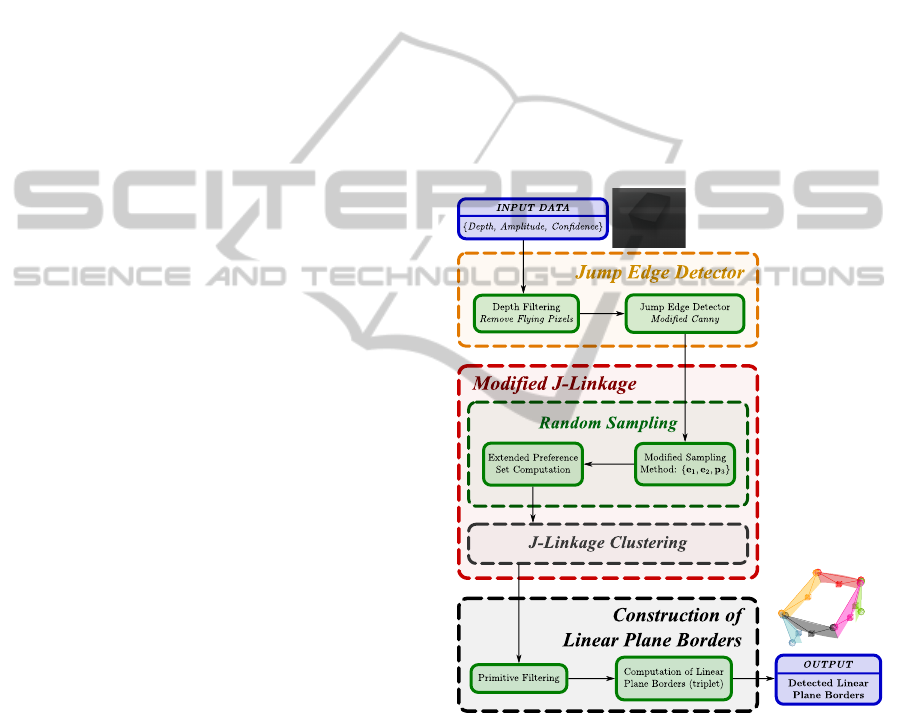
paper proposes a pipeline consisting of three stages,
illustrated in Fig. 1.
Figure 1: General diagram of the proposed detection of
Linear Plane Borders. {e
1
, e
2
, p
3
} represent the sampled
points needed to calculate a LPB hypothesis: two edge
points and one point in the correct face of the linear edge.
1. Jump Edge Detector. This stage detects depth
discontinuities which are the clue of finding edges
of geometrical objects. The process is carefully
designed to deal with noise and depth artifacts that
usually appear around such discontinuities.
2. Modified J-Linkage. J-Linkage is an algorithm
that groups together points based on the
consistency with randomly sampled model
LinearPlaneBorder-APrimitiveforRangeImagesCombiningDepthEdgesandSurfacePoints
461

hypotheses. In our case, each LPB hypothesis is
created by sampling two jump edge points likely
belonging to the same plane border and a third
point that is far enough from the edge but at a
distance limited by the LPB width.
3. Construction of LPBs. After running J-Linkage,
points in the depth image are grouped in different
LPBs hypotheses. This stage refines the LPBs
using linear least squares fit produce an accurate
estimate of the three points used to parameterize
each LPB.
3 PROPOSED METHOD
Each of the three aforementioned stages of our
method are detailed next.
3.1 Jump Edge Detector
In this paper, a jump edge is defined as a
depth discontinuity that produces an edge in the
depth image. Detecting jump edges properly
in depth images is not trivial. In most of
depth-image technologies (specially ToF cameras),
depth measurements are highly unstable around
jump edges, producing artifacts commonly known as
“flying pixels” or ”veil points” (see Fig. 2). The
detection of jump edges is performed in two steps:
1. Depth Filtering: this step implements a very
simple statistical filter, described by Rusu et al.
(2008), to detect “flying pixels”. It is based on
comparing the statistical distribution of depths
around each pixel. Once detected, they are filtered
out, using the depths of their neighboring pixels.
2. Canny-based Edge Detector: Lejeune et al.
(2011) proposed a modified magnitude of the
depth gradient for use in the Canny edge
detector which considers the uncertainty of depth
measurements, characterized for the physical
device used to compute depth. We use their
version that is specifically designed for ToF
cameras. If depth filtering is not performed
before the Canny detector, “flying pixels” will be
highlighted by the filter, giving erroneous depths
in the edges.
Fig. 2 shows the result of the “jump edge” detector
in a real scene. After this step, “jump edge” gradient
magnitude ∇D(p) and gradient direction ∇
φ
(p) are
obtained. The Canny detector performs binary
segmentation of ∇D so that jump edge candidates can
be easily found.
3.2 Modified J-Linkage
The core of our method is a modified version of the
J-Linkage algorithm, originally proposed by Toldo
and Fusiello (2008), to group points in the depth
image into different LPB hypotheses.
In a nutshell, J-Linkage can be explained in three
steps: first, n hypotheses (models) from the input
data (e.g. depth image) are selected randomly using
minimal set solutions (two points for a line, three
points for a plane, ...). Second, each point in the
input set is classified according to its distance to each
model. All models compatible with a point form the
so-called preference set of that point. Each point
forms its own cluster. Third, the clusters of points
with similar preference sets are merged together,
keeping only the models in the preference set of
a cluster that are compatible with all of its points.
The algorithm stops when all clusters have disjunct
preference sets.
We propose modifications to the two first steps
of J-Linkage so that LPBs are efficiently detected
given an input depth image and the resulting jump
edge detection detailed in the previous section.
Instead of randomly selecting three points to construct
plane hypotheses, our approach makes use of a
semi-deterministic procedure to sample these three
points leading to a reduction of the n hypothesis that
have to be generated. Preference sets for every point
are computed by applying an extended test to adjust
planar models to the proposed LPBs.
3.2.1 Random Sampling Stage
We propose a new random sampling strategy to
create n LPB hypotheses from the input depth image.
Although LPBs are indeed plane structures (minimal
set of three points), they must be attached to linear
jump edges. We sample sets of only two points, in
image coordinates, belonging to jump edges, namely
(e
1
,e
2
). These two points must be close enough to
belong to the same edge, and far enough to produce
a stable LPB hypothesis. The required third point
is determined from the other two in a deterministic
way that is explained below. In this way, the original
method proposed by Toldo and Fusiello (2010) for
detecting planes with J-Linkage is sped up.
The detailed steps to obtain a single random LPB
hypothesis from the input data are:
1. Sample uniformly a jump edge point (e
1
),
where e
1
is a two-dimensional point in image
coordinates.
2. Sample an edge point (e
2
) with the following
conditional probability function:
VISAPP2013-InternationalConferenceonComputerVisionTheoryandApplications
462

Figure 2: Detection of jump edges and flying-pixel removal. From left to right, we show the detected jump edges (white
points) in the depth image, the corresponding point cloud before the flying-pixels removal (jump edges are tagged as red
points) and the point cloud after removing flying-pixels.
p(e
2
|e
1
) =
p
close
if ke
1
− e
2
k ∈ (δ
1
,δ
2
) and |∇
φ
(e
1
) − ∇
φ
(e
2
)| < δ
φ
p
med
if ke
1
− e
2
k ∈ (δ
1
,δ
2
) and |∇
φ
(e
1
) − ∇
φ
(e
2
)| > δ
φ
p
f ar
if ke
1
− e
2
k /∈ (δ
1
,δ
2
)
where p
f ar
< p
med
<< p
close
and the interval
(δ
1
,δ
2
) establishes the lower and upper Euclidean
distances between e
1
and e
2
so that they can
be considered compatible neighbors. The values
∇
φ
(e
1
) and ∇
φ
(e
2
) represent the local jump edge
orientation at points e
1
and e
2
, respectively.
Hence, e
2
is chosen with the highest probability
(p
close
) if its distance with respect e
1
is inside
the interval (δ
1
,δ
2
) and the difference between
their edge orientations is smaller than δ
φ
. If
only the distance condition is met, e
2
is chosen
with a smaller probability (p
med
). If none of the
conditions is met, then point e
2
is chosen with the
smallest possible probability (p
f ar
).
In order to speed up searching for candidates of
e
2
, a k-Nearest Neighbor tree is built.
3 The selection of the third point (p
3
) is computed
in a deterministic way. We find p
3
by selecting the
point that is at a distance d from the middle point
of the line connecting e
1
and e
2
, where d is half
the length of the line. This leaves two possibilities
for point p
3
. We use the depth to select the point
closest to the camera as the solution (see Fig. 3).
Figure 3: Overview of the modified ramdom sampling
stage.
4 Compute the normal plane equations, denoted
as Π, of the LPB using the 3D points
(Q(e
1
),Q(e
2
),Q(p
3
)).
As it is shown in Section 4 the new sampling
method speeds up the random sampling stage and
provides sufficient flexibility for the generation of the
primitives that could support the correct LPBs.
3.2.2 Preference Set Computation
From the previous step, a set of n LPB models has
been obtained:
M = {m
1
,··· , m
n
} where m
i
= (Π
i
,e
i
1
,e
i
2
,p
i
3
)
(1)
Given a point p from the input data, the preference
set of p, namely PS(p) consists of the set of sample
models p is compatible with. It can be computed as
the intersection of the following three sets (see Fig. 4
for a graphical representation):
• A = {m
i
s.t. d
plane
Q(p),Π
i
} < ε, where
d
plane
is the distance from the point Q(p) to the
plane Π
i
,
• B = {m
i
s.t. d
edge
Q(p)
Π
i
,Q(e
i
1
),Q(e
i
2
)
< L},
where d
edge
is the distance from the projection of
Q(p) in the plane Π
i
to the edge formed by Q(e
i
1
)
and Q(e
i
2
), and
• C = {m
i
s.t. D(p) < D(p
Π
i
)}.
Finally, the preference set of point p is given as:
PS(p) = A ∩ B ∩C . (2)
3.3 Construction of Linear Plane
Borders
After J-Linkage terminates, each cluster of points
corresponds to an LPB hypothesis. In this section we
detailed how these clusters are actually parameterized
with a refined LPB of a proper length and width. A
LPB is mathematically defined as the triplet created
by two points corresponding to the bounds in the
edge segment and one point corresponding to the
maximum width of the “stripe” (see Fig. 5).
LinearPlaneBorder-APrimitiveforRangeImagesCombiningDepthEdgesandSurfacePoints
463
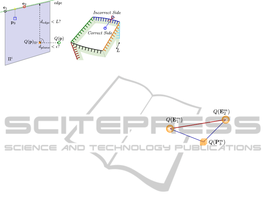
Test A, B
Test C
Figure 4: Tests applied to compute the preference set of
every point.
3.3.1 Primitive Filtering
Extending the initial J-Linkage proposal, we consider
that outliers to the new primitive not only emerge as
small cluster in the number of points but also in the
width of the stripe that they support. In order to avoid
non desirable LPBs, depending on the application, we
apply rejection thresholds in:
• minimum number of points, and
• minimum width.
By definition, a LPB must be supported by some
edge points, so that if there is any clustering that do
not hold any edge point it will also be discarded as a
correct primitive.
3.3.2 Primitive Definition
Let m be the number of primitives after the filtering
method, then LPBs are constructed as follows:
• For LPB
m
, compute the two boundary edge points
(Q(E
m
1
), Q(E
m
2
)):
1. Consider all the edge points that belong to
LPB
m
.
2. Compute the plane that best fits all the points
belonging to LPB
m
using linear least squares.
As edge points are noisy measurements, other
methods like jointly fitting the edge line and the
plane could degenerate.
3. Project all the edge points onto the best fitted
plane, previously computed.
4. Apply Principal Component Analysis (PCA) to
compute the first two principal directions.
5. Calculate the minimum and maximum values
along the principal components and extract the
boundary points.
6. Reproject the boundary points onto the original
coordinate frame to get the edge limits of
LPB
m
: (Q(E
m
1
), Q(E
m
2
))
• Compute the representative plane point (Q(P
m
3
)):
1. Obtain the equation of the 3D line created by
{Q(E
m
1
), Q(E
m
2
)}.
2. Project all the points belonging to LPB
m
into
the best fitted plane, previously computed.
3. Calculate the distance of every projected point
to the 3D edge line and select the maximum
distance (wd
max
).
4. Compute the two points at distance wd
max
from
the middle of the segment {Q(E
m
1
), Q(E
m
2
)} in
the perpendicular direction.
5. Select the point in the correct side by checking
for the one that has a nearer point in LPB
m
:
(Q(P
m
3
)).
Figure 5: Conceptual representation of a LPB.
4 EXPERIMENTS AND RESULTS
This section tests the detection of LPBs in real scenes
captured with a commercial ToF camera. We compare
LPB detection, as it is proposed in this paper against
a state-of-art plane fitting using J-Linkage.
In Fig. 6, we show 7 different scenes composed
of planar structures and the result of each step of
the algorithm. We also add the result of detecting
planes with J-Linkage where input data have been
re-sampled in a 1:4 ratio (one of each two columns
and rows), so that the number of input data is
comparable in both approaches. In these experiments,
the number of J-Linkage random samples are around
{5000−7000} for LPB and almost ten times more for
planes.
As quantitative results we show the accuracy of
LPB detection in Table 1. Ground-truth data are
obtained by manual annotation over the depth images
so that the different planes it is composed of are
clearly identified. Error is measured as the mean of
the Euclidean distance between points projected onto
the ground-truth plane and the projection onto the
plane obtained in LPBs detection.
It is clearly shown that LPB detection is
very accurate, capturing very useful geometric
information. It is also faster than detecting only
planes as it is shown in Table 2.
In a qualitative manner we show in Fig. 7 the
VISAPP2013-InternationalConferenceonComputerVisionTheoryandApplications
464
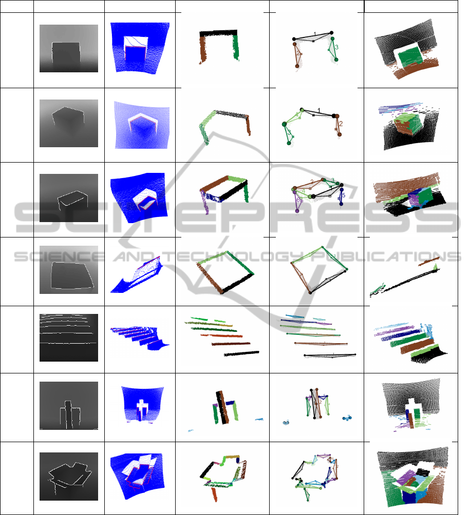
Example Jump Edges (2D) Jump Edges (3D) LPB JLinkage LPB Construction
JLinkage for Planes
1
2
3
4
5
6
7
Figure 6: Comparison between the detection of planes using the original JLinkage method and the main stages of the LPB
algorithm presented in this paper.
results with curved objects (non planar objects can
also be approximated as an arrangement of LPBs).
While these scenes are not piece-wise planar, LPB
detection is giving useful and stable information.
5 CONCLUSIONS
This paper shows that LPBs can be efficiently
detected in depth images, taken with a comercial
depth sensor of real man-made scenes composed of
planar structures.
LinearPlaneBorder-APrimitiveforRangeImagesCombiningDepthEdgesandSurfacePoints
465
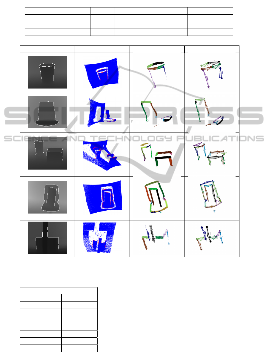
Table 2: Achieved speed-up for the main consuming processes.
Achieved Speed-Up
Example 1 2 3 4 5 6
7
Random
Sampling
x124.5 x103.5 x101.2 x78.3 x48.2 x85.6
x74.5
Clustering x8.8 x23.1 x6.1 x4.7 x1.8 x9.1
x5.4
Jump Edges (2D) Jump Edges (3D) JLinkage for LPBs
LPB Construction
Figure 7: Qualitative results for curved objects in more complex scenarios.
Table 1: Plane detection accuracy using LPB.
Plane Detection Accuracy
Example
Proposal
1
0.00123253
2
0.00176433
3
0.00192681
4
0.00280092
5
0.00795743
6
0.00384587
7
0.00461953
The proposed semi-deterministic sampling
method for LPBs allows to perform J-Linkage with
ten times less hypothesis than general plane fitting
methods. This reduction has a critical impact on the
algorithm’s speed.
As it can be seen in the results, LPBs are able
to capture rich information about the objects in the
scene compared to looking only for planar structures.
It also behaves reasonably well in curved objects.
In future works, edges due to changes in plane
orientations that are not detected now as jump edges
will be included. These additional edges will increase
VISAPP2013-InternationalConferenceonComputerVisionTheoryandApplications
466

the number of LPBs that can be obtained from a
geometric object. We also believe that LPBs can
be extended to curved objects, using curved stripes
attached to jump edges.
REFERENCES
Bartoli, A. (2007). A random sampling strategy for
piecewise planar scene segmentation. Computer Vision
and Image Understanding, 105(1):42–59.
Comaniciu, D. and Meer, P. (2002). Mean shift: A
robust approach toward feature space analysis. Pattern
Analysis and Machine Intelligence, IEEE Transactions
on, 24(5):603–619.
Feng, C., Deng, F., and Kamat, V. R. (2010).
Semi-automatic 3D reconstruction of piecewise planar
building models from single image. The 10th
International Conference on Construction Applications
of Virtual Reality.
Fiolka, T., St
¨
uckler, J., Klein, D., Schulz, D., and Behnke,
S. (2012). Sure: Surface entropy for distinctive 3d
features. Spatial Cognition VIII, pages 74–93.
Fischler, M. and Bolles, R. (1981). Random sample
consensus: a paradigm for model fitting with
applications to image analysis and automated
cartography. Communications of the ACM,
24(6):381–395.
Fouhey, D., Scharstein, D., and Briggs, A. (2010). Multiple
plane detection in image pairs using J-Linkage. In Proc.
ICPR–2010.
Jim
´
enez, D., Pizarro, D., Mazo, M., and Palazuelos,
S. (2012). Modelling and correction of multipath
interference in time of flight cameras. In Computer
Vision and Pattern Recognition (CVPR), 2012 IEEE
Conference on, pages 893–900. IEEE.
Lange, R. and Seitz, P. (2001). Solid-state time-of-flight
range camera. Quantum Electronics, IEEE Journal of,
37(3):390 –397.
Lejeune, A., Pierard, S., Van Droogenbroeck, M., and
Verly, J. (2011). A new jump edge detection method for
3D cameras. International Conference on 3D Imaging
(IC3D).
May, S., Dr
¨
oschel, D., Fuchs, S., Holz, D., and Nuchter,
A. (2009). Robust 3D-mapping with time-of-flight
cameras. In Intelligent Robots and Systems, 2009. IROS
2009. IEEE/RSJ International Conference on, pages
1673–1678. IEEE.
Redondo-Cabrera, C., Lopez-Sastre, R.,
Maldonado-Bascon, S., and J., A.-R. (2012). SURFing
the point clouds: Selective 3D spatial pyramids
for category-level object recognition. In 2012
IEEE Conference on Computer Vision and Pattern
Recognition, pages 3458–3465. IEEE.
Rusu, R., Marton, Z., Blodow, N., Dolha, M., and Beetz,
M. (2008). Towards 3D point cloud based object maps
for household environments. Robotics and Autonomous
Systems, 56(11):927–941.
Schwarz, L., Mateus, D., Lallemand, J., and Navab, N.
(2011). Tracking planes with time of flight cameras
and J-Linkage. In IEEE Workshop on Applications of
Computer Vision (WACV), 2011, pages 664–671. IEEE.
Shotton, J., Fitzgibbon, A., Cook, M., Sharp, T., Finocchio,
M., Moore, R., Kipman, A., and Blake, A. (2011).
Real-time human pose recognition in parts from single
depth images. In CVPR, volume 2, page 7.
Smisek, J., Jancosek, M., and Pajdla, T. (2011). 3D
with kinect. In Computer Vision Workshops (ICCV
Workshops), 2011 IEEE International Conference on,
pages 1154–1160. IEEE.
Steder, B., Rusu, R., Konolige, K., and Burgard, W. (2011).
Point feature extraction on 3D range scans taking into
account object boundaries. In Robotics and Automation
(ICRA), 2011 IEEE International Conference on, pages
2601–2608. IEEE.
Taguchi, Y., Tuzel, O., Liu, M.-Y., and Ramalingam,
S. (2012). Voting-based pose estimation for robotic
assembly using a 3d sensor. In Robotics and Automation
(ICRA), 2012 IEEE International Conference on, pages
1724–1731. IEEE.
Toldo, R. and Fusiello, A. (2008). Robust multiple
structures estimation with J-Linkage. Computer
Vision–ECCV 2008, pages 537–547.
Toldo, R. and Fusiello, A. (2010). Real-time incremental
J-Linkage for robust multiple structures estimation.
In International Symposium on 3D Data Processing,
Visualization and Transmission (3DPVT).
Xu, L., Oja, E., and Kultanen, P. (1990). A new curve
detection method: randomized hough transform (rht).
Pattern Recognition Letters, 11(5):331–338.
Zhang, W. and Kosecka, J. (2007). Nonparametric
estimation of multiple structures with outliers.
Dynamical Vision, pages 60–74.
Zuliani, M., Kenney, C., and Manjunath, B. (2005). The
multiransac algorithm and its application to detect planar
homographies. In Image Processing, 2005. ICIP 2005.
IEEE International Conference on, volume 3, pages
III–153. IEEE.
LinearPlaneBorder-APrimitiveforRangeImagesCombiningDepthEdgesandSurfacePoints
467
