
Statistical Inverse Lighting
Eduardo Fern
´
andez
1
and Gonzalo Besuievsky
2
1
Centro de C
´
alculo, Universidad de la Rep
´
ublica, Montevideo, Uruguay
2
Geometry and Graphics Group, Universitat de Girona, Girona, Spain
Keywords:
Inverse Lighting, Radiosity.
Abstract:
Inverse lighting techniques allows to obtain the unknown light sources parameters, such as light position or
flux emission, from desired lighting intentions. In this paper we present a new inverse lighting technique that
uses the statistical mean and variance of the illuminated scene to obtain optimal solutions for a given lighting
intention. This technique allows to explore a huge number of full radiosity solutions in a short time, reducing
in this way drastically the optimization time required.
1 INTRODUCTION
Lighting intentions (LI) are the goals that designers
would like to achieve in the illumination design pro-
cess. Given an interior space to illuminate, this pro-
cess achieves several steps that goes from the use of
the space to the specific light accentuation to be ob-
tained (Russell, 2008). Once the LIs are specified the
designer provides the set of parameters that must ful-
fill the intentions. Then, the light positions, shape and
power of the emitters, must be selected.
The management of all lighting parameters is a
huge combinatorial problem. Usually, to find a so-
lution, the problem is treated as an inverse method.
That is, a method where the illumination aspects are
unknown and must be determined. The whole process
involves two main computational tasks: the global il-
lumination simulation and the search of an optimal
solution. The first one is crucial to obtain accurate
lighting information. For the second one, an opti-
mization process is used to fulfill the requirements.
Most of the previous work on inverse lighting for
global illumination problems provides good numer-
ical methods, omitting timing considerations, which
can be a problem for interactive design.
In this paper we present a new inverse lighting
method, that focus on the use of statistical LI and
that greatly improves timing of previous work. Our
main contribution is to introduce a new technique
that relates LIs to the lighting mean and variance of
the scene. Our method exploits coherence of inte-
rior spaces to build a compact radiosity representa-
tion that is efficiently used to quickly explore many
lighting solutions. We present previous work is in
Section 2 and the background for lighting represen-
tation we used in Section 3. Our statistical approach
is introduced in Section 4 and test results are shown
in Section 5. Finally, conclusions and future work are
summarized in Section 6.
2 PREVIOUS WORK
One of the first attempts to infer emitter positions
and shapes given lighting intentions, is presented in
(Schoeneman et al., 1993) through the intuitive prin-
ciple of ”Painting with light”, but where the interac-
tivity is achieved only for direct illumination. In our
work we are focusing on indirect illumination.
In the context of radiosity, several works driven by
different motivations and assumptions were proposed.
A survey on all these methods can be found in (Patow
and Pueyo, 2003). In (Contensin, 2002), an Inverse
Radiosity method based on a pseudo-inverse of the
radiosity matrix is formulated. Kawai et al. (Kawai
et al., 1993) perform the optimization over the intensi-
ties and directions of a set of lights, as well as surface
reflectivity, in order to best convey the subjective im-
pression of certain scene qualities expressed by users.
In (Castro et al., 2012), an heuristic search algorithm
combined with linear programming is used to opti-
mize light positioning with an energy-saving goal.
In all inverse lighting methods the coherence is
used to improve the global illumination computation.
In (Castro et al., 2012), a re-using random walk paths
technique is employed. They store an irradiance ma-
185
Fernández E. and Besuievsky G..
Statistical Inverse Lighting.
DOI: 10.5220/0004297501850190
In Proceedings of the International Conference on Computer Graphics Theory and Applications and International Conference on Information
Visualization Theory and Applications (GRAPP-2013), pages 185-190
ISBN: 978-989-8565-46-4
Copyright
c
2013 SCITEPRESS (Science and Technology Publications, Lda.)

trix that allows computing, for each patch of the scene
the power contribution of fixed light points. We based
our work on the low-rank radiosity method (LRR)
(Fern
´
andez, 2009), that allows to obtain a full radios-
ity solution in real time with changing lighting param-
eters and small computer storage.
Our work deals also with optimization problems.
These problems consists of finding the best solution
from all of the feasible solutions, which are defined
through a set of constraints. For illumination pur-
poses, each constraint is related to a lighting intention
for all or part of the scene. To find an optimal solu-
tion, heuristic approach are used, which avoid visit-
ing the whole search space. There are a large number
of heuristic search algorithms in the literature, which
can potentially be used to solve lighting problems
(hill climbing, beam search and simulated annealing)
(Russell and Norvig, 2003). In (Castro et al., 2012)
a wide range of these algorithms are explored. In
(Cassol et al., 2011) and (Schneider et al., 2009), the
scenes are simplified to rectangular spaces, and the
inverse problem is solved through a generalized ex-
tremal optimization approach. In (Fern
´
andez and Be-
suievsky, 2012), the Variable Neighborhood Search
(VNS) method (Hansen and Mladenovic, 2001) was
used. We also used VNS for the present work.
3 COMPACT LIGHTING
REPRESENTATION
Lighting intentions (LI) are defined as goals that de-
signers must provide to achieve the desired illumina-
tion. Designers can set many LI. Examples of LIs
are: ”Guarantee a minimum of irradiance in a panel
in order to be seen correctly” or ”Distribute the light
homogeneously over all surfaces” (Figure 1).
In the discrete radiosity problem, the radiosity of
the scene is computed by solving the linear system
shown in Eq. 1 (Cohen et al., 1993).
(I − RF)L
B
= E (1)
where I is the identity matrix with dimension n×n (n
is the number of patches), R is a diagonal matrix that
stores the reflectivity of the patches, F is the form fac-
tors matrix, L
B
is a vector with the radiosity values,
and E is the emission vector. The designer goal is to
find E (to configure the position and radiosity values
of the light sources), so that L
B
meets all LI.
Usually the F matrix is not computed, due to
memory constraints. The n×n matrix M of Eq. 2 also
has high order of complexity, so is rarely computed.
L
B
= ME (2)
Figure 1: A top-view scene with a lighting intention config-
uration example (top) and a possible solution for position-
ing four light sources (bottom).
In this paper we use information from the M ma-
trix to define LIs, for this purpose, so we use the
low-rank radiosity (LRR) methodology (Fern
´
andez,
2009). In LRR the matrix F is aproximated by the
product of two matrices (UV
T
), with dimension n×k
(nk). The O(nk) memory needed, allows storing U
and V
T
in the main memory. This work also exposes
an approximation of the M matrix (see Eq. 3) intro-
ducing Y, which is also a n×k matrix.
L
B
= ME ∼
I − YV
T
E (3)
where Y = −RU
I − V
T
RU
−1
4 STATISTICAL BASED LI
In statistics (Canavos, 1984), the mean (µ) and the
standard deviation (σ) are used to describe properties
about sets of numerical data. µ describes the central
tendency of the data and σ measures their dispersion.
In this paper is used µ and σ to describe LIs. We show
that µ(L
B
(s)) and σ(L
B
(s)) could be obtained without
the previous calculation of L
B
(p) for patches p be-
longing to the scene s. Here we explain the calcula-
tion process of µ and σ, and how can be used in LI.
GRAPP2013-InternationalConferenceonComputerGraphicsTheoryandApplications
186

4.1 Mean (µ) of L
B
(s)
Radiosity is defined as light flux per unit of surface,
so it is the mean (weighted by the area of the patches)
of the flux density on all patches (Eq. 4).
µ(L
B
(s,E)) =
∑
p∈s
W
A
(i,i)L
B
(p,E) =
(1
T
s
W
A
M)E = V
L
B
(s) · E (4)
In Eq. 4, W
A
is a diagonal matrix with weights
(W
A
(i,i) = A(i,i)/
∑
j
A( j, j)). V
L
B
(s)
is a n×1 vector.
In the calculation of the radiosity on a static
scene the vector V
L
B
(s) does not varies. In summary,
µ(L
B
(s)) can be computed with complexity O(n), us-
ing a single dot product.
4.2 Standard Deviation (σ) of L
B
(s)
The standard deviation (σ) is a scale parameter which
determines the dispersion of a data set. Any radios-
ity vector can be interpreted as a list of sample data
of a “random variable L
B
” which varies on a surface.
Figure 2 shows an E-shaped scene with five different
configurations of lights. Each L
B
has its own σ(L
B
)
value, which measures the dispersion of the radiosity
values along each scene. The more homogeneously
illuminated the scene, the lower σ(L
B
) associated, be-
cause of the small dispersion of the L
B
lighting values.
(a) σ = 0.43 (b) σ = 1.03 (c) σ = 1.52
(d) σ = 2.1 (e) σ = 3.51
Figure 2: Different radiosity distributions in the ”E” scene
(n=24736), and their σ values. Red patches are the emitters.
To speed up the calculation of σ(L
B
), we consider
L
B
as a linear combination of random variables: the
vector L
B
can be defined as a linear combination of
the M columns (Eq. 5):
L
B
= ME =
∑
i
M(:,i)E(i) (5)
where M(:,i) is the sample data of an i
th
random vari-
able. Also is important the relation between the vari-
ance and the covariances, as expressed in Eq. 6.
var(
∑
i
L
i
a
i
) =
∑
i j
cov(L
i
,L
j
)a
i
a
j
, (6)
In Eq. 6, L
i
and L
j
are random variables, a
i
and a
j
are
constants, and cov is the covariance between L
i
and
L
j
. Then, Eqs. 5 and 6 can be combined as:
var(L
B
) = var(
∑
i
M(:,i)E(i)) =
∑
i j
cov(M(:,i),M(:, j))E(i)E( j) = E
T
cov(M)E (7)
In equation Eq. 7, cov(M) is a n×n covariance ma-
trix, where each element cov(M)(i, j) is the covari-
ance associated with the i
th
and j
th
variables of M
(with sample data M(:,i) and M(:, j)).
4.3 Low-rank Covariance Matrix
In Eq. 7, cov(M) concentrates all geometric infor-
mation, so, when the geometry is static it can be cal-
culated in a precomputation stage. But an impor-
tant drawback of this equation is the O(n
2
) memory
needed to store cov(M). Fortunately, because of the
lighting coherence in the scenes, the correlation be-
tween lighting data of close patches is high, so the
cov(M) is a numerically low-rank matrix. Figure 3
shows the covariance matrix and its singular value de-
composition (SVD) of a Cornell box. It can be appre-
ciated that cov(M) has many pairs of similar rows.
The plot of the SVD values (Figure 3 (b)) confirms
that it is composed with redundant information.
To build a smaller covariance matrix, we replace
the matrix M in Eq. 7 by its low-rank variant YV
T
(Eq. 3) producing a k×k covariance matrix (Eq. 8).
var(L
B
) ∼ var(YV
T
E) =
var(
∑
i
Y(:,i)(V
T
E)
i
) = (V
T
E)
T
cov(Y)(V
T
E) (8)
In this equation (V
T
E) is k×1 and (V
T
E)
i
is the i
th
el-
ement. Also, each column Y(:,i) contains the sample
values of a random variable. Finally, cov(Y) is the
k×k covariance matrix associated to those variables.
A brute force calculation of var(L
B
) using Eq. 8
consumes O(nk) operations. This result is higher than
the complexity obtained for µ calculation. As stated
in (Fern
´
andez et al., 2012), for any scene with coarse
and fine-grained meshes, it is possible to built a sparse
StatisticalInverseLighting
187
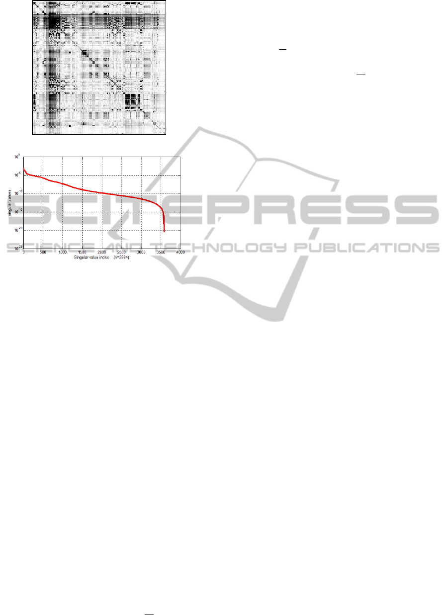
(a) cov(M(s,:)) (white ≡ 0 value).
(b) Singular values of cov(M(s,:)).
Figure 3: Covariance matrix and its SVD decomposition for
a Cornell box with 3584 patches.
matrix V such that the complexity of V
T
E product
could be reduced to O(n). So, through a careful use of
Eq. 8, the complexity of the variance can be reduced
to O(n + e
2
) where e is the number of emitter patches
in the coarse-grained mesh.
4.4 Chebyshev’s based Constraints
A designer may want to optimize the lighting scene
using certain LI, wishing to minimize the consump-
tion of artificial light, but also bounding the light lev-
els or the contrast. All these LI can be transformed
into optimization goals and constraints, using µ and
σ parameters. For instance, to control a given con-
straint to be fulfilled (L
min
≤L
B
(p)∀p ∈ s), we have to
calculate all the L
B
(p) values, which has complexity
O(nk). A O(n) option consists in finding µ(L
B
(s))
and σ(L
B
(s)) to bound the probability of any p to ful-
fill the constraint. The inequation 9 shows a new con-
straint formulation, where the parameter a establishes
the probability of success in the transformation.
L
min
≤ µ(L
B
(s)) − aσ(L
B
(s)) (9)
To explain the meaning of a, we base our reason-
ing in the Chebyshev’s inequality (Canavos, 1984):
P[aσ(L
B
(s)) ≤ |µ(L
B
(s)) − L
B
(p)|] ≤
1
a
2
,∀p ∈ s
where P is the probability function. This inequality is
fulfilled for any L
B
independently of their distribution.
It can be demonstrated that when the new constraint
is fulfilled, the probability of failure in the original
constraint is
1
a
2
(Inequation 10).
P[L
B
(p) ≤ L
min
] ≤
1
a
2
(10)
This result is a probabilistic approach, and as such,
does not guarantees certainty whatsoever. The new
constraint built is a worst case boundary, meaning that
smaller values of a also can provide good results.
5 TEST RESULTS
We built three experiments for solving inverse light-
ing problems. For the first one we aim to demonstrate
the use of the variance as a LI. In the second one,
we analyze the method changing statistical parame-
ters for optimization. Those experiments have an av-
erage time execution of 10s for each run, and each
experiment is carried out 20 times, totalizing 200s.
Finally, a performance comparison of the proposed
method with other methods is evaluated. All simu-
lations were performed in a Matlab environment on a
notebook computer (Intel Core i7-2670QM 2.2 Ghz
processor with Turbo Boost up to 3.1 Ghz and 4 GB
DDR3 memory).
Our optimization engine is based on the Vari-
able Neighborhood Search (VNS) method (Hansen
and Mladenovic, 2001). VNS is a single-solution
based metaheuristic that finds global optimum solu-
tions. However, we believe that similar results could
be achieved with another optimization engine.
5.1 Dispersion
In this experiment we show the use of σ to manage
the distribution of the light in the scene.
Scene: “E” corridor (s
Ec
). (n×k)=(24736×1546).
Goal: We seek to illuminate the scene in a uniform
manner, positioning six diffuse light sources.
LI Goal Translation: min σ(L
B
(s
Ec
)).
Constraints Translation: i) Six emitters. ii) Emit-
ters are located in the installation area e (the red-
colored rectangle in Figure 1). iii) The radiosity
value of emitters is unique and predefined.
Variables: 12. Six 2D coordinates that delimit the
location of the light sources.
Running Details: i) The precomputation of Y, V,
and cov(Y), to apply the Eq. 8, takes about 12
GRAPP2013-InternationalConferenceonComputerGraphicsTheoryandApplications
188
minutes. ii) The VNS algorithm is executed 20
times. iii) 25000 evaluations of σ on each run,
totalizing half a million evaluations.
Results: i) Min, max, and mean of the σ values
found: 0.425, 0.442, and 0.430. ii) Sample image:
Figure 2 (a). Figures 2 (b), (c), and (d) were found
adding to this experiment a constraint (σ ≥ k), and
changing the value of k for each image. Figure 2
(e) was found changing the goal to max σ(L
Br
(s)).
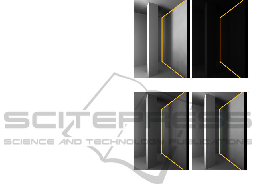
5.2 Statistical Tools for LI
In this experiment we analyze the convenience of us-
ing µ and σ to satisfy a wide variety of LI. The ex-
periment is developed on the same scene and with the
same implementation than the previous one. Four dif-
ferent LI aspects were tested on a specific wall of the
scene (the “yellow-colored wall” in Figure 1).
L
Illuminate
Goal: to illuminate the wall as much as possible, po-
sitioning six diffuse light sources.
LI Goal Translation : max µ(L
B
(s
Y w
)).
Results: Min, max, and mean of the µ values found:
0.394, 0.427, and 0.420. See Figure 4 (a).
L
Overshadow
Goal: to overshadow the wall as much as possible.
LI Goal Translation: min µ(L
B
(s
Y w
)).
Results: Min, max, mean of µ values: 7.2×10
−4
,
7.64×10
−4
, 7.38×10
−4
. See Figure 4 (b).
L
Disseminate
Goal: to disseminate homogeneously the light over
the wall, within radiosity boundaries.
LI Goal Translation: min σ(L
B
(s
Y w
)).
LI Constraint Translation: .30≤µ(L
B
)≤.35.
Results: Min, max, and mean of the σ values found:
0.066, 0.073, and 0.067. See Figure 4 (c).
L
Contrast
Goal: the highest contrast illumination as possible in
the wall, within radiosity boundaries.
LI Goal Translation: max σ(L
B
(s)).
LI Constraint Translation: .30≤µ(L
B
)≤.35.
Results: Min, max, and mean of the σ values found:
0.159, 0.175, and 0.171. See Figure 4 (d).
(a) max µ(=.442) (b) min µ(=7e − 4) (the image
shows L
B
×50)
(c) min σ(=.066) subject to
.30≤µ(L
B
)≤.35
(d) max σ(=.175) subject to
.30≤µ(L
B
)≤.35
Figure 4: Four LI configurations applied to the “yellow-
colored wall” (see Figure 1).
5.3 Chebyshev-based Constraints
In this experiment we test the new constraint built
(see Ineq. 9), minimizing µ(L
B
(p)) and replacing
L
min
=0.1≤L
B
(p), ∀p ∈“colored-yellow wall” with
L
min
=0.1≤µ(L
B
(s))−aσ(L
B
(s)).
Three values were tested for the parameter a: 1,
2, and 3 (see Figures 5 (a), (b), and (c)). According
to Chebyshev, a = 3 means that less than 1/9 of all
patches have values below 0.1, but the test shows a
better result, because no patch is below the boundary.
5.4 Performance Comparison
The statistical inverse lighting method (SIL) allows
to evaluate half a million µ and σ in less than four
minutes. This result greatly improves previous work.
We compare this result performing the same test with
two different inverse lighting approaches, as used in
(Fern
´
andez and Besuievsky, 2012): using the full
LRR method and using LRR but computing only the
radiosity at the wall (LRR+) (see Table 1).
StatisticalInverseLighting
189
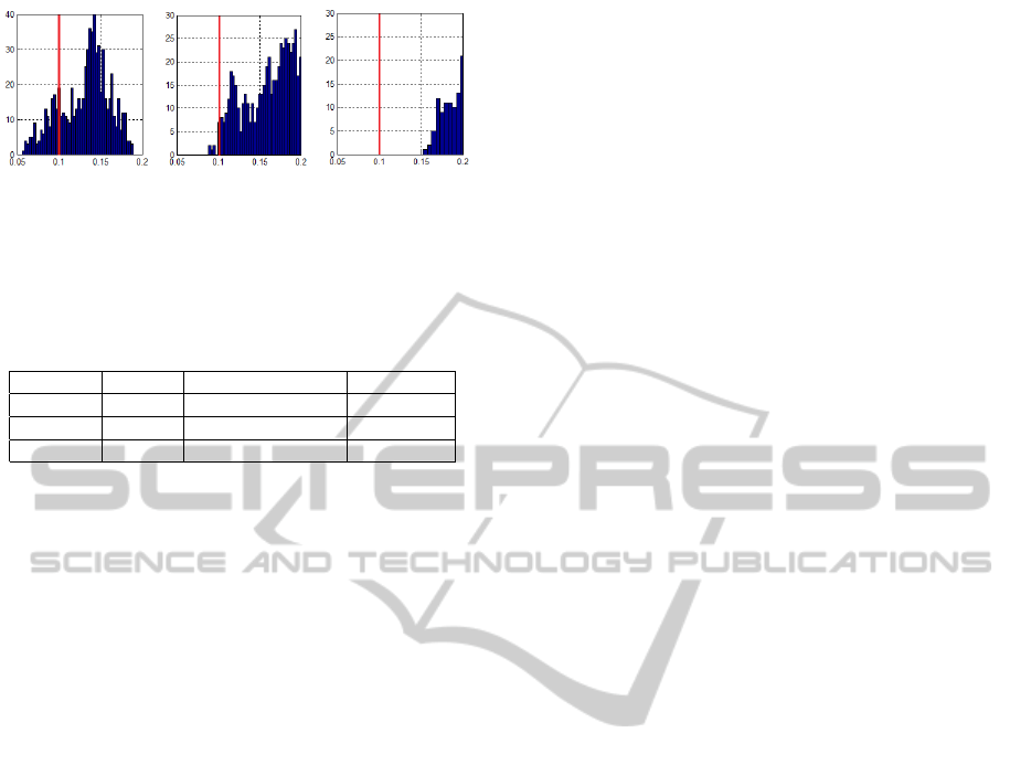
(a) .1 ≤ µ−σ. (µ=.13,
σ=.026).
(b) .1 ≤ µ−2σ. (µ=.17,
σ=.034).
(c) .1 ≤ µ−3σ. (µ=.30,
σ=.063).
Figure 5: The LI (minµ(L
B
(s) subject to .1≤L
B
) is modeled
with three values of a (from left to right: a=1, 2, and 3).
Table 1: Comparative of optimization approaches against
our statistical technique.
Method Tests/s Total time (min) Speed-Up
SIL 2083 4 -
LRR+ 59 141 35
LRR 8 1041 260
6 CONCLUSIONS AND FUTURE
WORK
In this paper is presented a new methodology for
achieving LI for inverse lighting problems. Our ap-
proach is based on the use of µ and σ as statistical pa-
rameters for the lighting values. Using a low-rank for-
mulation, we demonstrate that µ and σ for L
B
can be
computed in O(n) and O(n + e
2
). This result allows
to perform thousands of global illumination evalua-
tion on a desktop PC, reducing drastically the over-
all optimization time required. We believe that this
technique could open a new avenue in the search for
optimal inverse lighting solutions. The results shown
could lead to the use of the method in more complex
scenes with more elaborated lighting intentions. Re-
lated to further development, more effort should be
focus on an automatic parametrization of the LI.
ACKNOWLEDGEMENTS
This work was partially funded by Programa de
Desarrollo de las Ciencias B
´
asicas (Uruguay) and
by grant TIN2010-20590-C02-02 from Ministerio de
Ciencia e Innovaci
´
on (Spain).
REFERENCES
Canavos, G. (1984). Applied probability and statistical
methods. Little, Brown.
Cassol, F., Schneider, P. S., Franc¸a, F. H., and Neto, A.
J. S. (2011). Multi-objective optimization as a new
approach to illumination design of interior spaces.
Building and Environment, 46(2):331 – 338.
Castro, F., del Acebo, E., and Sbert, M. (2012). Energy-
saving light positioning using heuristic search. En-
gineering Applications of Artificial Intelligence,
25(3):566 – 582.
Cohen, M., Wallace, J., and Hanrahan, P. (1993). Radiosity
and realistic image synthesis. Academic Press Profes-
sional, Inc., San Diego, CA, USA.
Contensin, M. (2002). Inverse lighting problem in radiosity.
Inverse Problems in Engineering, 10(2):131–152.
Fern
´
andez, E. (2009). Low-rank radiosity. In Rodr
´
ıguez,
O., Ser
´
on, F., Joan-Arinyo, R., and J. Madeiras,
J. Rodr
´
ıguez, E. C., editors, Proceedings of the IV
Iberoamerican Symposium in Computer Graphics,
pages 55–62. Sociedad Venezolana de Computaci
´
on
Gr
´
afica, DJ Editores, C.A.
Fern
´
andez, E. and Besuievsky, G. (2012). Inverse lighting
design for interior buildings integrating natural and ar-
tificial sources. Computers & Graphics, 36(8):1096–
1108.
Fern
´
andez, E., Ezzatti, P., Nesmachnow, S., and Be-
suievsky, G. (2012). Low-rank radiosity using sparse
matrices. In Proceedings of GRAPP2012, pages 260–
267.
Hansen, P. and Mladenovic, N. (2001). Variable neighbor-
hood search: Principles and applications. European
Journal of Operational Research, 130(3):449–467.
Kawai, J. K., Painter, J. S., and Cohen, M. F. (1993). Ra-
dioptimization - goal based rendering. In ACM SIG-
GRAPH 93, pages 147–154, Anaheim, CA.
Patow, G. and Pueyo, X. (2003). A survey of inverse render-
ing problems. Computer Graphics Forum, 22(4):663–
688.
Russell, S. (2008). The Architecture of Light: Architectural
Lighting Design, Concepts and Techniques: a Text-
book of Procedures and Practices for the Architect,
Interior Designer and Lighting Designer. Concept-
nine.
Russell, S. J. and Norvig, P. (2003). Artificial Intelligence:
A Modern Approach. Pearson Education, 2 edition.
Schneider, P. S., Mossi, A. C., Franca, F. H. R., de Sousa,
F. L., and da Silva Neto, A. J. (2009). Application of
inverse analysis to illumination design. Inverse Prob-
lems in Science and Engineering, 17(6):737–753.
Schoeneman, C., Dorsey, J., Smits, B., Arvo, J., and Green-
berg, D. (1993). Painting with light. In Proceedings of
the 20th annual conference on Computer graphics and
interactive techniques, ACM SIGGRAPH 93, pages
143–146, New York, NY, USA. ACM.
GRAPP2013-InternationalConferenceonComputerGraphicsTheoryandApplications
190
