
Using n-grams Models for Visual Semantic Place Recognition
Mathieu Dubois
1,2
, Emmanuelle Frenoux
1,2
and Philippe Tarroux
2,3
1
Univ Paris-Sud, Orsay, F-91405, France
2
LIMSI-CNRS, B.P. 133, Orsay, F-91403, France
3
´
Ecole Normale Sup
´
erieure, 45 Rue d’Ulm, Paris, F-75230, France
Keywords:
Semantic Place Recognition, Hidden Markov Models, n-grams.
Abstract:
The aim of this paper is to present a new method for visual place recognition. Our system combines global
image characterization and visual words, which allows to use efficient Bayesian filtering methods to integrate
several images. More precisely, we extend the classical HMM model with techniques inspired by the field
of Natural Language Processing. This paper presents our system and the Bayesian filtering algorithm. The
performance of our system and the influence of the main parameters are evaluated on a standard database. The
discussion highlights the interest of using such models and proposes improvements.
1 INTRODUCTION
Semantic mapping (see (N
¨
uchter and Hertzberg,
2008)) is a relatively new field in robotics which aims
to give the robot a high-level, human-compatible, un-
derstanding of its environment in order to ease the
integration of robots in daily environments, notably
homes or workplaces. Such environments are usu-
ally composed of discrete places which correspond to
different functions. For instance a house is usually
made of different rooms and corridors used to move
between them. Such places are called semantic places
because they are defined in high-level human con-
cepts as opposed to traditional low-level landmarks
used in robot mapping.
In this context, it’s important for the robot to be
able to recognize in which place or category of places
it lies. Those tasks are called respectively instance
recognition and categorization. Semantic place recog-
nition is then an important component of semantic
mapping. Moreover the semantic category of a place
can be used to foster object detection and recognition
(giving priors on objects identity, location and scale)
and to provide qualitative localization.
Different types of sensors have been employed for
semantic place recognition. The first works in this do-
main used range sensors to discriminate places based
on geometrical information. However the spatial con-
figuration of two places of the same category (e.g. two
kitchens) can be very different. Therefore geomet-
rical information may not be useful for categoriza-
tion. Vision is the modality of choice for semantic
place recognition because it gives access to rich, al-
lothetic information. Although there are multimodal
approaches, our work focuses on visual place recog-
nition.
In this article we will further develop an anal-
ogy between semantic place recognition and language
modelling. This analogy allows to design efficient
temporal integration methods i.e. to take several im-
ages into account in order to reduce ambiguity. More
precisely, we will extend the Hidden Markov Model
(HMM) formalism with n-grams models. Those mod-
els have been extensively used in Natural Language
Processing (NLP) and efficient estimation techniques
have been proposed. This paper aims to assess the use
of such models in semantic place recognition. The
goal is to compare this temporal integration method
to previously proposed models. In particular we will
study the influence of the length of the n-gram model
and estimation procedure on performance.
The article is structured as follows. Section 2
presents related work. Our model and its links with
language modelling are described in section 3. Sec-
tion 4 presents our experiments and the results. Fi-
nally we conclude in section 5.
2 RELATED WORK
Some authors (see (Vasudevan et al., 2007)) use an
object-based approach. In this case they employ a
808
Dubois M., Frenoux E. and Tarroux P..
Using n-grams Models for Visual Semantic Place Recognition.
DOI: 10.5220/0004298708080813
In Proceedings of the International Conference on Computer Vision Theory and Applications (VISAPP-2013), pages 808-813
ISBN: 978-989-8565-47-1
Copyright
c
2013 SCITEPRESS (Science and Technology Publications, Lda.)

standard algorithm for object localization and recog-
nition. Places are described by the frequency of ob-
jects found in them combined with constraints on
their position. However, object categorization is
still a difficult task and the position of objects can
greatly vary from one environment to another. There-
fore those approaches have not been used on large
databases.
The vast majority of research on place recognition
use techniques developed for visual scene classifica-
tion. We can distinguish methods using global fea-
tures (see (Torralba et al., 2003)) and methods using
descriptors computed around interest points (see (Ul-
lah et al., 2008)). (Filliat, 2008) uses the Bag-of-
Words (BoW) model: local features are first clustered
into a so-called dictionary of visual words learned by
mean of a vector quantization algorithm. An image is
represented by the distribution of visual words found
in it. The major advantage is that the learning space
is discretized but all geometrical information is lost.
Generally speaking using a single image or a sin-
gle type of information is not enough for place recog-
nition tasks. Therefore a lot of research has been con-
ducted to disambiguate perception. (Pronobis and Ca-
puto, 2007) use a confidence criterion to iteratively
compute several cues from the same image until con-
fidence in the classification is sufficiently high (or no
more cues are available).
Another method to reduce ambiguity is to use
several images to mutually disambiguate perception.
In (Pronobis et al., 2010), the authors use a sim-
ple spatio-temporal accumulation process to filter the
decision of a discriminative confidence-based place
recognition system (which uses only one image to
recognize the place). One problem with this method
is that the system needs to wait some time before giv-
ing a response. Also, special care must be taken to
detect places boundaries and to adjust the size of the
bins. (Torralba et al., 2003) use a HMM where each
place is a hidden state and the feature vector stands for
the observation. The drawback is that the input space
is continuous and high-dimensional. The learning
procedure is then computationally expensive. (Ran-
ganathan, 2010) uses a technique called Bayesian on-
line change-point detection. The main idea is to de-
tect abrupt changes in the parameters of the input’s
statistics caused by moving from one place to another.
The main advantage is that the robot is able to learn
in an unsupervised way but relies on the hypothesis
that the shape of the distribution is the same for every
place.
Several works (see (Wu et al., 2009; Guillaume
et al., 2011; Dubois et al., 2011)) have combined
global image description and vector quantization. In
this case, each image is described by a single vi-
sual word. The sequence of images is then trans-
lated into a sequence of words. Such techniques al-
low to draw a parallel between place recognition and
language modelling. (Wu et al., 2009) propose to
use a HMM with discretized signatures. Temporal
integration is performed with Bayesian filtering (see
section 3). (Dubois et al., 2011) propose to use an
extended model called auto-regressive HMM to take
into account the dependence between images.
In this paper we push this idea a step further. The
next section presents our models and its relations to
the standard HMM model.
3 PLACE RECOGNITION WITH
n-GRAMS
Our model is similar to the one described in (Guil-
laume et al., 2011; Dubois et al., 2011). Each image is
described by a unique feature vector which is mapped
to a given visual word thanks to a vector quantiza-
tion algorithm (see section 3.3). The main novelty lies
in the use of High-Order Hidden Markov Model (see
section 3.1) and techniques for visual word selection
(see 3.4).
3.1 High-order Hidden Markov model
In HMMs the relationship between x
t
, the robot’s
knowledge of the world at time t, and z
t
, its per-
ception is represented by figure 1(a). In the case
of place recognition, the state is a discrete random
variable which represents the place the robot is in
at time t. In this model, each place c
i
∈ C is
modelled by the continuous probability distribution
p(z
t
|x
t
= c
i
). This formalism allows to efficiently es-
timate the a posteriori probability bel(x
t
) = P(x
t
|z
1:t
)
by a recursive equation (see (Wu et al., 2009)) given
the discrete place transition probability distribution
P(x
t
|x
t−1
) which encodes the topology of the envi-
ronment.
It is assumed that the current observation depends
only on the current hidden state i.e. that the state is
complete. However, there is a huge semantic gap be-
tween the human notion of a place and what can be
extracted from an image. Several authors have pro-
posed extensions of the classic HMM to take into ac-
count long-term dependencies between observations
(see (Berchtold, 2002; Lee and Lee, 2006)). In this
paper we will call this model High-Order Hidden
Markov Model (HOHMM). In this case, the current
knowledge x
t
depends on the last ` states x
t−`:t−1
.
Similarly the current observation z
t
depends on x
t
and
Usingn-gramsModelsforVisualSemanticPlaceRecognition
809

the n previous observations z
t−n:t−1
(see figure 1(b)).
In this paper we restrict ourselves to the case ` = 1.
Therefore the state transition matrix is unchanged.
The a posteriori distribution bel(x
t
) is given by:
bel(x
t
) = p (z
t
|z
t−n:t−1
,x
t
)
∑
c
i
∈C
P(x
t
|x
t−1
)bel(x
t−1
)
(1)
The place model is given by the distribution
p(z
t
|z
t−n:t−1
,x
t
= c
i
). This probability distribution
may be very difficult to learn because it is continu-
ous.
3.2 HOHMM and Visual Words
In order to simplify learning of the place model (Guil-
laume et al., 2011; Dubois et al., 2011) have pro-
posed to use global image characterization in com-
bination with vector quantization algorithms to dis-
cretize them. In this case the variable z
t
is reduced
to a discrete random variable with a finite number of
values
{
1,...,K
}
where K is the number of words in
the dictionary.
In this case, the model of place c
i
is
given by the discrete probability distribution
P(z
t
|z
t−n:t−1
,x
t
= c
i
). In NLP, such a model is
known as a n + 1-gram model because it uses n + 1
words. (Chen and Goodman, 1996) have shown that
the estimation of the model from empirical data is
an important factor. One problem is that even with
a large training set, some sequences of words will
not be observed in training data for a given class and
therefore they will be assigned a null probability in
this class’ model. If such a sequence is observed in
the testing set then the a posteriori probability of this
class will be clamped to 0 due to equation 1. To avoid
this problem, it is necessary to take some probability
mass from the observed sequences and distribute
it to unobserved sequences. Those techniques are
called smoothing or discounting. We refer the
reader to (Manning and Sch
¨
utze, 1999) for a unified
presentation of smoothing techniques. We use the
SRILM toolkit to learn the n-grams models.
3.3 Image Characterization and Vector
Quantization
To characterize the images we use the GIST descrip-
tors (see (Torralba et al., 2003)) which is an efficient
global image characterization. The image is divided
into 4 × 4 subwindows (we use only the luminance
channel) and filtered using a bank of Gabor filters (we
use 4 scales and 6 orientations). The energy of the
filter is then averaged on each subwindow for each
scale and orientation. Finally the output is projected
on the first 80 principal components which explains
more than 99% of the variance. Thus this descriptor
captures the most significant spatial orientations at a
given scale.
The vector quantization algorithm used in this pa-
per is the Self-Organizing Map (SOM) (see (Koho-
nen, 1990)). In the current set-up the training of
the SOM is performed off-line on a set of randomly
chosen images made of
1
/3 of the COLD DB. The
number of neurons on the map sets the number of
words in the visual dictionary which is an impor-
tant parameter of the system. We use square maps
parametrized by their length S (therefore K = S
2
). In
this paper we will use S = 10 and S = 20. Those
values were selected because it has been shown that
small maps have a good performance on categoriza-
tion tasks while larger maps perform well for instance
recognition (see (Guillaume et al., 2011)). Because
the training algorithm is stochastic, the results vary
from one SOM to another. Therefore for each size S,
the results are averaged for 5 SOMs.
3.4 Visual Words Selection
The sampling rate of most databases is several Hertz.
In this case, image at time t + 1 is not very different
from image at time t and there is a high probability
that they are described by close vectors and therefore
by the same visual word. While this is a desirable
feature of image description and vector quantization,
this may be a problem for our method because the
probability of seeing the same visual word than before
will be very high. Therefore it might be interesting to
use only a subset of the images (and then the words)
for learning.
In order to evaluate this phenomenon we have
computed the average number of consecutive time-
steps which are characterized by the same visual word
for the training sequence used in section 4. Results are
given in table 1.
We will test three different strategies for selecting
visual words. The first one is simply to sub-sample
the input image i.e. to select 1 image out of s (s is the
sub-sampling rate). This strategy will be called “sub-
sample”. The second strategy is to replace every se-
quence of m identical prototypes by a unique instance
of this word (m is the compression rate). We will call
this strategy “compress”. The last strategy is to use
the word at time t only if it is different than the word at
time t − 1. We will call this strategy “unique”. Those
strategies are simple and can be implemented online
on a real robot with limited computational power.
In the next section we will present the experiment
we carried out to study the use of this model for se-
VISAPP2013-InternationalConferenceonComputerVisionTheoryandApplications
810
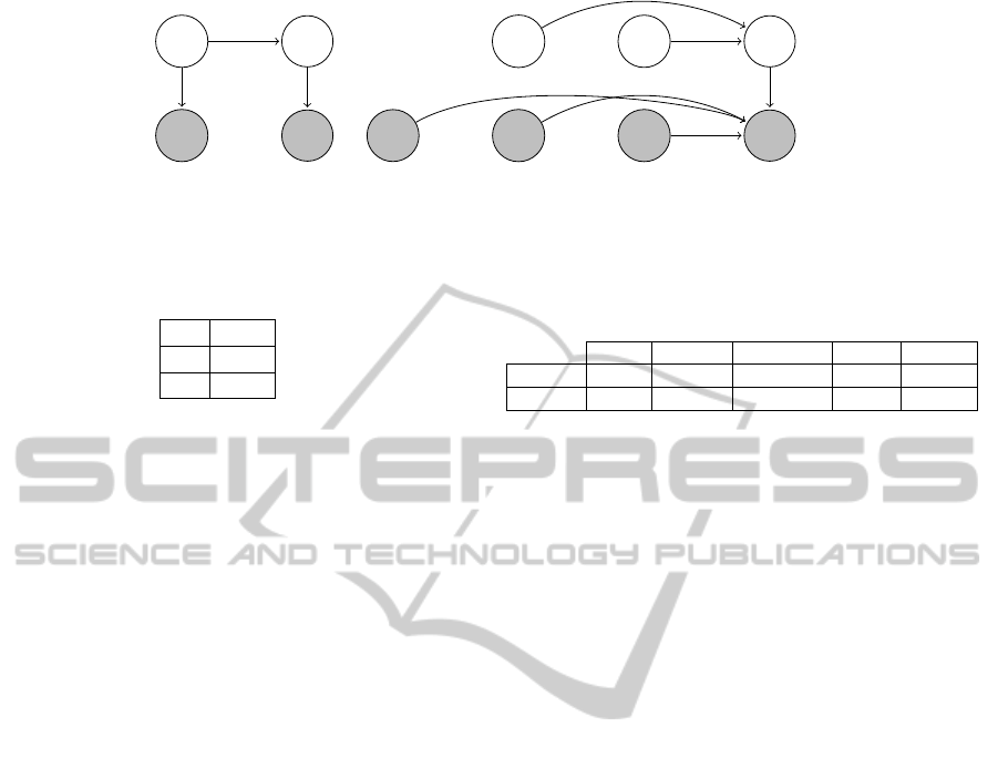
X
t−1
X
t
Z
t−1
Z
t
(a)
X
t−`
X
t−1
X
t
...
Z
t−n
Z
t−2
Z
t−1
Z
t
...
(b)
Figure 1: (a) The classical HMM model. (b) The HOHMM model (we only show nodes that have an influence on x
t
and z
t
).
Table 1: Average number of consecutive images represented
by the same visual word for different SOM size.
S
¯
t
10 3.15
20 2.67
mantic place recognition.
4 EXPERIMENTAL RESULTS
4.1 Experimental Design
We use the COLD database (see (Ullah et al., 2008))
a standard database to evaluate vision-based place
recognition systems. It consists of sequences ac-
quired by a human-driven robot in different labora-
tories across Europe under different illumination con-
ditions (night, cloudy, sunny). In each laboratory, two
paths were explored (standard and extended). Each
path was followed at least 3 times under each illu-
mination condition. All the experiments were carried
out with the perspective images.
Protocols proposed by (Ullah et al., 2008) uses
only a few hundreds images per place which is not
enough to robustly estimate the transition probabil-
ities. Therefore we designed a new experiment to
evaluate the interest of our method. We use only im-
ages acquired in Saarbruecken part B because other
parts of the database are known to contain errors (e.g.
missing places or labellisation errors) or are not com-
plete (e.g. only one path was followed). There are
five classes (see table 2). Training is performed with
sequences number 1 and 2 from all the three illumina-
tion conditions. Similarly, testing is performed with
sequence 3 from all the illumination conditions.
Following (Wu et al., 2009) we define the transi-
tion matrix as P (x
t
|x
t−1
) = p
e
if x
t
= x
t−1
; the rest
of the probability mass is shared uniformly among all
other transitions. We use p
e
= 0.99.
In order to test the influence of the n-gram order
we have varied n between 1 and 6. Similarly we have
tested the Lidstone-Laplace (LL) smoothing with pa-
Table 2: Number of images for each category in the training
and testing sets. There are 11,380 training and 5,192 testing
images.
Office Corridor Printer area Toilets Kitchen
Training 1,375 4,464 1,190 3,272 1,079
Testing 606 1,964 532 1,513 577
rameter δ = 1 and the Witten-Bell (WB) smoothing.
The training set was too small to use the Knesser-Nay
smoothing. In our experiments we use interpolated
models (Manning and Sch
¨
utze, 1999). We have tested
several values of the sub-sampling rate: s = 1 (which
has no effect), s = 3 and s = 5. We use m = 3 for
the “compress” strategy. The “unique” strategy don’t
need any parameter.
Setting n = 1 with Lidstone-Laplace smoothing
gives the same temporal integration method than
in (Wu et al., 2009) (note that we don’t use the
same signature). Setting n = 2 with Lidstone-Laplace
smoothing and without interpolation gives a system
similar to (Dubois et al., 2011).
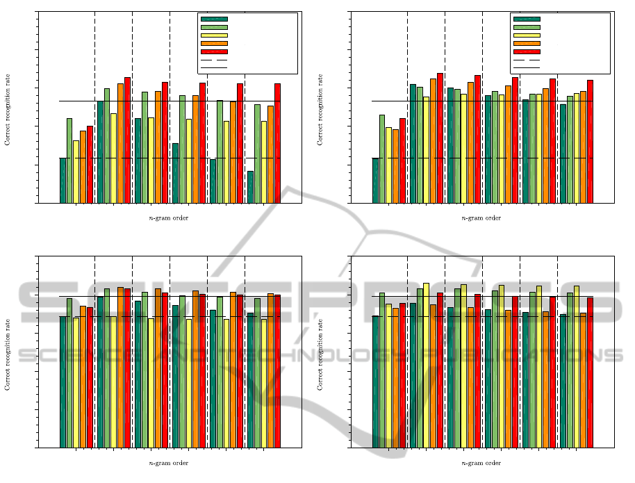
4.2 Results
Results are presented on figure 2. It must be noted
that on this instance recognition task, a larger SOM
gives better results. This is expected from the litera-
ture (see (Guillaume et al., 2011)). The second obser-
vation that could be made is that the word selection
methods generally increase the results by several per-
cent. This can be seen by the difference between the
bar for s = 1 and other bars of the same group. The
“subsample” strategy with s = 3 is rather efficient,
sometimes increasing performance by 6%. Setting
s = 5 generally gives less important increase. Per-
formance decreases with S = 20 and LL smoothing.
However, this strategy leads to the best results on the
task for S = 20 and WB smoothing. The “compress”
strategy is usually efficient except for s = 20 and WB
smoothing. The “unique” strategy is always among
the best choices and it’s results are less sensitive to the
n-gram order. Generally speaking, the effect of those
strategies increase with n. Results with WB smooth-
ing are generally a little bit better than with LL in par-
Usingn-gramsModelsforVisualSemanticPlaceRecognition
811
subsam ple s= 1
subsample s= 3
subsample s= 5
com press
unique
Wu et al., 2009
Dubois et al., 2011
0.65
0.70
0.75
0.80
0.85
0.90
1 2 3 4 5 6
(a) S = 10, Lidstone-Laplace smoothing
subsample s= 1
subsample s= 3
subsample s= 5
com press
unique
Wu et al., 2009
Dubois et al., 2011
0.65
0.70
0.75
0.80
0.85
0.90
1 2 3 4 5 6
(b) S = 10, Witten-Bell smoothing
0.65
0.70
0.75
0.80
0.85
0.90
1 2 3 4 5 6
(c) S = 20, Lidstone-Laplace smoothing
0.65
0.70
0.75
0.80
0.85
0.90
1 2 3 4 5 6
(d) S = 20, Witten-Bell smoothing
Figure 2: Results on the instance recognition task. The vertical axis is the correct recognition rate (in %). The horizontal axis
is the value of n. Upper-row: results for S = 10. Lower row: results for S = 20. Left column: results for Lidstone-Laplace
smoothing. Right column: results for Witten-Bell smoothing.
ticular for large n.
It is clear from the figure that using n = 2, i.e. to
take into account the dependence on the last image,
is a clear improvement over n = 1, i.e. the classical
HMM. However using n-grams with n > 2 has little
impact on performance. It should be noted that when
s = 1, the performance drops when n > 2. With word
selection, the performance can be high with large n.
This seems to confirm the intuition behind the word
selection techniques.
5 CONCLUSIONS
We have presented a new model of temporal integra-
tion using HOHMM for semantic place recognition
which models the dependence between observations.
We have shown that taking this dependence into ac-
count can lead to interesting gains in performance.
However, contrary to what we expected, using larger
n don’t improve performance. The smoothing tech-
nique seems to have minor effect. This may be caused
by the fact that we use relatively small training sets
compared to the field of NLP where those techniques
have been developed. Those results must take into ac-
count the fact that recognition rates are already quite
high on the task studied here.
We have shown that simple methods to select im-
portant words could improve the results. Our results
suggest that large n could be interesting if combined
with good word selection techniques.
Future works will focus on the vector quantiza-
tion process to learn better words. More sophisticated
word selection techniques may also be useful. Finally
we could also look for more discriminative descrip-
tors.
VISAPP2013-InternationalConferenceonComputerVisionTheoryandApplications
812

ACKNOWLEDGEMENTS
We thanks Thiago Fraga and Alexandre Allauzen for
fruitful discussion and help with the SRILM toolkit.
REFERENCES
Berchtold, A. (2002). High-order extensions of the double
chain markov model. Technical Report 356, Univer-
sity of Washington.
Chen, S. F. and Goodman, J. (1996). An empirical study of
smoothing techniques for language modeling. In Pro-
ceedings of the 34th annual meeting on Association
for Computational Linguistics.
Dubois, M., Guillaume, H., Tarroux, P., and Frenoux, E.
(2011). Visual place recognition using bayesian fil-
tering with markov chains. In Proceedings of the
European Symposium on Artificial Neural Networks
(ESANN 2011).
Filliat, D. (2008). Interactive learning of visual topological
navigation. In Proceedings of the 2008 IEEE Interna-
tional Conference on Intelligent Robots and Systems
(IROS 2008).
Guillaume, H., Dubois, M., Tarroux, P., and Frenoux, E.
(2011). Temporal Bag-of-Words: A Generative Model
for Visual Place Recognition using Temporal Integra-
tion. In Proceedings of the International Conference
on Computer Vision Theory and Applications (VIS-
APP 2011).
Kohonen, T. (1990). The self-organizing map. In Proceed-
ings of the IEEE, volume 78, pages 1464–1480.
Lee, L.-M. and Lee, J.-C. (2006). A study on high-order
hidden markov models and applications to speech
recognition. In Ali, M. and Dapoigny, R., editors, Ad-
vances in Applied Artificial Intelligence, volume 4031
of Lecture Notes in Computer Science.
Manning, C. and Sch
¨
utze, H. (1999). Foundations of statis-
tical natural language processing. MIT Press.
N
¨
uchter, A. and Hertzberg, J. (2008). Towards semantic
maps for mobile robots. Robotics and Autonomous
Systems, 56(11):915–926.
Pronobis, A. and Caputo, B. (2007). Confidence-based cue
integration for visual place recognition. In Procced-
ings of the 2007 IEEE/RSJ International Conference
on Intelligent Robots and Systems.
Pronobis, A., Mozos, O. M., Caputo, B., and Jenseflt, P.
(2010). Multi-modal semantic place classification.
The International Journal of Robotics Research, 29(2-
3):298–320.
Ranganathan, A. (2010). PLISS: Detecting and labeling
places using online change-point detection. In Pro-
ceedings of the 2010 Robotics: Science and Systems
Conference (RSS 2010).
Torralba, A., Murphy, K. P., Freeman, W. T., and Rubin.,
M. A. (2003). Context-based vision system for place
and object recognition. In Proceedings of the Nineth
IEEE International Conference on Computer Vision
(ICCV 2003), volume 1, pages 273–280.
Ullah, M. M., Pronobis, A., Caputo, B., Luo, J., Jensfelt, P.,
and Christensen, H. I. (2008). Towards robust place
recognition for robot localization. In Proceedings of
the IEEE International Conference on Robotics and
Automation (ICRA 2008), Pasadena, USA.
Vasudevan, S., Gachter, S., Nguyen, V., and Siegwart, R.
(2007). Cognitive maps for mobile robots–an object
based approach. Robotics and Autonomous Systems,
55(5):359–371.
Wu, J., Christensen, H., and Rehg, J. (2009). Visual
place categorization: Problem, dataset, and algorithm.
In IEEE/RSJ International Conference on Intelligent
Robots and Systems, 2009 (IROS 2009).
Usingn-gramsModelsforVisualSemanticPlaceRecognition
813
