Robust Guided Matching and Multi-layer Feature Detection

Applied to High Resolution Spherical Images

Christiano Couto Gava, Alain Pagani, Bernd Krolla and Didier Stricker

German Research Center for Artiﬁcial Intelligence, Trippstadter Straße 122, Kaiserslautern, Germany

Keywords:

Robust Guided Matching, Feature Detection, Spherical Imaging, 3D Reconstruction, Multi-view Stereo.

Abstract:

We present a novel, robust guided matching technique. Given a set of calibrated spherical images along with

the associated sparse 3D point cloud, our approach consistently ﬁnds matches across the images in a multi-

layer feature detection framework. New feature matches are used to reﬁne existing 3D points or to add reliable

ones to the point cloud, therefore improving scene representation. We use real indoor and outdoor scenarios

to validate the robustness of the proposed approach. Moreover, we perform a quantitative evaluation of our

technique to demonstrate its effectiveness.

1 INTRODUCTION

The need for generation of accurate 3D models of

objects and scenes is increasing as technologies for

three-dimensional visualization become more popu-

lar and accessible. In this scenario, computer vision

algorithms play a fundamental role. Speciﬁcally, 3D

reconstruction techniques are a promising instrument

to support promotion, training, games or education.

Nowadays, image-based reconstruction algo-

rithms are able to produce models of small objects

that can compete with those produced by laser scan

techniques (Schwartz et al., 2011), (N¨oll et al., 2012).

These methods demand a highly controlled environ-

ment for capturing the images, particularly concern-

ing lighting conditions. Thus they are not suitable for

reconstructing scenes in out-of-lab situations.

Nevertheless, reconstruction of large scenes is

an attractive tool for documentation, city planning,

tourism and preservation of cultural heritage sites

(Hiep et al., 2009), (Furukawa et al., 2010), (Pagani

et al., 2011). In this context, several reconstruction

approaches adopt a region growing strategy, in which

3D points are used as seeds and the scene is gradually

reconstructed as regions grow. However, this strategy

normally fails when the distance between seed points

is large and the ﬁnal reconstruction is incomplete.

In this paper we present a method that robustly

performs matching of image features to support multi-

view stereo (MVS) algorithms. Our approach is de-

signed to consistently create seeds and improve scene

sampling based on a novel guided matching tech-

nique. It beneﬁts from point clouds produced by

modern Structure from Motion (SfM) algorithms and

imposes a set of constraints to achieve robustness.

Moreover, we propose a multi-layer feature detection

method to allow hierarchical matching designed to

work with any choice of local feature descriptors.

We apply our algorithm to high resolution spheri-

cal images because it has been shown in (Pagani et al.,

2011) and (Pagani and Stricker, 2011) that they are

more suitable to perform SfM. Due to their wide ﬁeld

of view, these images provide more constraints on

camera motion as features are more often observed.

Therefore, spherical images are more qualiﬁed for

guided matching than standard perspective images.

Guided matching has been addressed by other re-

searchers. In (Triggs, 2001) the Joint Feature Dis-

tributions (JFD) are introduced. JFD form a general

probabilistic framework for muli-view feature match-

ing. The idea is to summarize the observed behaviour

of feature correspondences instead of rigidly con-

strain them to the epipolar geometry. Similar to our

work, the method yields conﬁdence search regions in-

stead of searching along the entire epipolar line. In

contrast, our approach explicitly combines 3D infor-

mation with epipolar geometry to deﬁne search re-

gions of higher conﬁdence.

The work presented in (Lu and Manduchi, 2004)

shares with ours the independence of image features

used for matching. Both methods only require a fea-

ture detector providing a local descriptor for each fea-

ture and a similarity function. However, Lu and Man-

duchi do not assume calibrated cameras. The method

322

Gava C., Pagani A., Krolla B. and Stricker D..

Robust Guided Matching and Multi-layer Feature Detection Applied to High Resolution Spherical Images.

DOI: 10.5220/0004300603220327

In Proceedings of the International Conference on Computer Vision Theory and Applications (VISAPP-2013), pages 322-327

ISBN: 978-989-8565-48-8

 2013 SCITEPRESS (Science and Technology Publications, Lda.)

was designed for the case of nearly parallel epipo-

lar lines, i.e. the epipoles are at inﬁnity. Thus it

would face challenging issues with spherical images,

because in this case the epipoles are always visible.

The paper is organized as follows: Section 2 in-

troduces the concept of spherical images and related

properties. Section 3 outlines our multi-layer feature

detection framework. The proposed robust guided

matching, our main contribution, is detailed is section

4. Experiments and results are discussed in section 5

and we conclude in section 6.

2 SPHERICAL IMAGES

Spherical images allow to register the entire scene

from a single point of view and may be acquired us-

ing dedicated hardware and software packages. Ac-

cording to the spherical geometry, each point on the

image surface deﬁnes a 3D ray r. Analogue to per-

spective imaging, given a 3D point P

in world co-

ordinate system (WCS), its counterpart in camera co-

ordinate system (CCS) is P

= RP

+ t, with R and

t representing the camera rotation matrix and transla-

tion vector. However, different from the perspective

case, the relationship between P

and its projection

p onto the image surface is simply P

= λp, with λ

being the depth of P

. Without loss of generality, we

assume a unit sphere, leading to kpk = 1. Thus, in

this case, the dehomogenization typical of perspective

images is not needed.

Epipolar Geometry. Consider a pair of spherical cam-

eras I

and I

. I

is regarded as reference while I

is re-

garded as target camera. Let R

and t

be the rotation

matrix and the translation vector from I

to I

. A point

on the surface of I

, along with the centers of the

cameras, deﬁne a plane Π, as seen in Figure 1. Π may

be expressed by its normal vector n

= R

×t

. For

any point p

on I

and belonging to Π the condition

= 0 holds. Thus Π is the epipolar plane deﬁned

by cameras I

and I

. This is the same result obtained

in the perspective case and it shows that the epipolar

constraint does not depend on the shape of image sur-

face. Nevertheless, to keep consistency with the 3D

scene captured by the images, not every point p

Π can be a match for p

. In fact, only those points

belonging to the arc deﬁned by p

and p

on Figure

1 may be considered for matching. Note that p

the epipole on I

and p

= R

. We refer to this arc

as epipolar arc.

Calibration of Spherical Cameras. Our approach

builds on (Pagani et al., 2011) and (Pagani and

Stricker, 2011). Thus, we assume the rotation ma-

trix R and the translation vector t for each camera are

known. Additionally we assume a set of 3D points

resulting from calibration is also provided. This set

may be seen as a coarse representation of the scene

and is referred to as Sparse Point Cloud (SPC).

Figure 1: Epipolar geometry of spherical images.

3 MULTI-LAYER FEATURE

DETECTION

In this section we focus on the automatic detection of

multiple feature layers. The method consists of hier-

archically detecting features, thus gradually increas-

ing image sampling. Here the main goal is to support

the robust guided matching, which will be detailed in

section 4.

Given an image I, a feature detector F and a pa-

rameter vector ρ controlling the behaviour of F , we

deﬁne a feature layer l as

l(I, F , ρ) = { f

u,v

| f

u,v

= F (I(u, v), ρ)}, (1)

where f

u,v

represents a feature detected on image I

with pixel coordinates (u, v). To improve readability

we will drop the subscripts of f

u,v

and refer to it as

f. l(I, F , ρ) may be seen as a vector of features, all

detected using the parameters ρ. Thus it is possible

to deﬁne for each image I a set of feature layers L by

varying ρ as

L(I, F , ρ

. . . ρ

K−1

) = {l

= l(I, F , ρ

)}, (2)

where k = 0, 1, .., K − 1 and K is the number of layers

to compute.

Furthermore, we set the parameters ρ

. . . ρ

K−1

produce layers with increasing number of features,

with the ﬁrst layer holding the most distinctive fea-

tures, i.e. the most reliable ones. If, instead of using

layers, a single large feature vector is computed, the

probability of ﬁnding the correct match decreases, be-

cause multiple similar features are usually found, i.e.

several ambiguous matches are stablished. This is the

main motivation to hierarchically create feature lay-

ers: They allow dense image sampling without affect-

ing calibration. In other words, with this hierarchical

approach, it is possible to:

1. obtain a precise calibration by employing only the

ﬁrst layer(s), i.e. using matches from the most dis-

tinctive features;

RobustGuidedMatchingandMulti-layerFeatureDetectionAppliedtoHighResolutionSphericalImages

323

2. improve performance as less matches need to be

computed for calibration;

3. combine as many layers as necessary to perform

robust guided matching.

In principle, any feature detector computing the lo-

cation of the feature on the image along with a lo-

cal descriptor of its neighborhood could be employed,

such as (Lowe, 2004), (Bay et al., 2008) or (Tola

et al., 2009). Additionally, a similarity function is re-

quired so that descriptors may be compared. In this

work, we employ the same feature detector as pro-

posed in (Pagani et al., 2011) and refer to it as Spher-

ical Afﬁne SIFT (SASIFT). SASIFT was chosen due

to its robustness against the distortion imposed by the

longitude-latitude representation of spherical images.

This is specially important near the image poles.

4 ROBUST GUIDED MATCHING

In this section the main contribution of our approach

is detailed. The goal is to robustly add 3D points to

the SPC to increase the number of seed points for

3D dense reconstruction or to improve the current

(sparse) representation of the scene.

Theoretically, an arbitrary number of layers could

be computed per image. In practice, few layers are

computed because this is already sufﬁcient to achieve

both precise calibration – using the ﬁrst layer – and

dense image sampling – using the remaining layers.

Yet, these layers may contain several thousands of

descriptors and handling numerous images simulta-

neously is not optimal as computational resources are

limited. Thus, we devise the method for pairs of im-

ages, so that only the corresponding layers have to be

handled. The image pairs are determined according to

their neighborhood relation, which is encoded in a bi-

nary upper triangular matrix N. If N(i, j) = 1, images

and I

are considered as neighbors and matches are

computed between them.

Our algorithm combines multiple feature layers,

3D points from calibration and a set of constraints,

as epipolar geometry, thresholding and symmetric

matching. Moreover, it enforces the consistency of

new 3D points and may be applied recursively, allow-

ing to push the number of points even further.

4.1 The Anchor Points

After calibration, most 3D points in the SPC are cor-

rectly triangulated. However, some outliers remain.

Thus, before applying our guided matching, outliers

are removed according to a local density computed

for each point in the SPC. We denote the ﬁltered point

cloud as S

. After ﬁltering, all remaining points are

assumed to be inliers. These points are regarded as

reference and we refer to them as anchor points. We

deﬁne an anchor point A as a 3D point in Euclidean

coordinates along with a set Θ holding the images and

the respective features where A is observed.

A =



∈ ℜ

Θ = {(I

, f) | λp = R

+ t

}

(3)

In Equation 3, p is the image point associated to f.

We also deﬁne the SPC as the set S of all anchor

points. To improve readability we sometimes use A

instead of its 3D coordinates P

throughout the text.

4.2 Matching based on Anchor Points

In the literature, the term guided matching is usually

regarded as the class of methods searching for corre-

spondences given a constraint. This constraint could

be imposed by epipolar geometry, a dispartity range

on aligned images, a predeﬁned or estimated search

region or any other criteria that restricts the search for

correspondences to a subset of the image pixels.

Our guided matching algorithm is not driven by a

single, but by a set of constraints, as described below.

Given a reference image I

, a target image I

, and a

feature f

detected on I

, we search for a feature f

under the following constraints:

1. Epipolar geometry: p

= 0, with E the essen-

tial matrix deﬁned by I

and I

, p

and p

are the

unit vectors corresponding to f

and f

;

2. Threshold: the matching score δ between the de-

scriptors of f

and f

is above a given threshold τ,

i.e. δ( f

, f

) > τ;

3. Symmetry: δ( f

, f

) is the highest score when

symmetric matching is performed, that is, f

and

are the best match when the roles of reference

and target images are swapped;

However, these constraints are usually not sufﬁ-

cient to achieve robust matching because the set of

features f

complying with the ﬁrst two criteria above

is in general large. As a result, the search has to be

done in a large set of potentially ambiguous features.

We propose an approach to overcome this is-

sue. Robustness of guided matching is improved by

combining the constraints outlined above, the anchor

points and a consistency ﬁlter. Our method works as

follows: For each feature f

a set of anchor points

projecting on a region Ω centered at p

is selected.

These points form a subset of S, S

Ω

. Assuming depth

continuity for the points in S

Ω

, they can be used to

determine a depth range [λ

min

, λ

max

] in which the 3D

VISAPP2013-InternationalConferenceonComputerVisionTheoryandApplications

324

point P

= λp

is expected to be. Consequently, the

points P

min

= λ

min

and P

max

= λ

max

deﬁne on the

epipolar arc on I

a conﬁdence region Ψ in which the

correct match f

is expected to be, as shown in Fig-

ure 2. This considerably reduces the search region

along the epipolar arc, thus increasing the likelihood

of ﬁnding the correct match. Then we apply the sec-

ond and third constraints described above to all fea-

tures in Ψ. Finally, the consistency ﬁlter is applied,

which will be detailed in section 4.4.

min

max

Ω

(a)

max

min

Ω

(b)

Figure 2: Determining the conﬁdence region Ψ based on

anchor points. The dots represent the subset S

Ω

. (a) Top

view and (b) Perspective view.

After applying the consistency ﬁlter we consider

the following 3 cases: 1. Ψ is empty; 2. Ψ contains

one feature; 3. Ψ contains two or more features. In

the ﬁrst case, as no reliable match has been found, the

algorithm moves on to match the next feature f

. For

the second case, a new anchor point is created and

added to S. Finally, if two or more features remain in

Ψ, we discard the matches to enforce robustness, i.e.

no anchor point is created.

4.3 Matching based on Apical Angles

The approach described above works for features f

whose S

Ω

0. If no anchor points project onto Ω, f

can not be matched based on anchor points. Increas-

ing the size of Ω does not necessarily solve the issue,

as the anchor points in S

Ω

may not be representative

of the true depth range.

We extend our approach to allow “isolated” fea-

tures to be matched. Here we do not use anchor points

to establish a depth range. Instead, we use apical an-

gles. Apical angle is the angle formed by rays ema-

nating from a 3D point towards the centers of the (pair

of) cameras where the 3D point is seen. Then, given

a minimum and a maximum apical angle, α

min

and

max

, the depth range is computed as follows. For a

feature f

, we compute the 3D points P

min

and P

max

so that the apical angles at P

min

and P

max

are α

max

and

min

, as shown in Figure 3. The conﬁdence region Ψ

is determined by the projections of P

min

and P

max

onto

and the rest of the matching proceeds as before.

max

min

max

Figure 3: Conﬁdence region Ψ based on apical angles.

4.4 The Consistency Filter

False matches yield 3D points that often violate the

ordering assumption. The Consistency Filter supports

guided matching by identifying such violations and is

explained as follows.

Consider a 3D query point P

resulting from the

triangulation of p

and p

. Let A be an anchor point

whose projections a

and a

onto I

and I

are in the

vicinity of p

and p

, respectively. The vectors p

and a

deﬁne a normal n

= p

× a

on I

. Similarly,

= p

× a

on I

. Given the rotation matrix R

, P

regarded as consistent if n

·R

> 0 holds for all an-

chor points projecting in the vicinity of p

and p

. Fig-

ure 4 shows this concept using a single anchor point.

(a)

(b)

Figure 4: Consistency ﬁlter. (a) P

is considered consistent

and (b) P

is considered inconsistent.

5 RESULTS

We applied our algorithm to several different datasets,

all captured with images of 100 MegaPixels (approx-

imately 14000 by 7000 pixels). Here we show two of

them: the Mogao Cave number 322 in China and the

Saint Martin Square in Kaiserslautern, Germany. We

processed these datasets on a machine equipped with

an Intel



Xeon



CPU W3520 @ 2.67GHz, 24 GB

of RAM, running Ubuntu 11.04 - 64 bits.

5.1 Overview

For all datasets we considered the ﬁrst feature layer

for calibration and all layers together for robust

matching. As mentioned in section 4.2, our algorithm

may be used recursively. We show this by applying

the matching based on anchor points in two steps. The

ﬁrst step takes as input the ﬁltered SPC S

and outputs

a SPC S

containing all points in S

along with the

new points. Analogously, the second step takes S

RobustGuidedMatchingandMulti-layerFeatureDetectionAppliedtoHighResolutionSphericalImages

325

input and delivers S

. We considered two parameters:

ﬁrst, a radius r to compute the region Ω centered at

the reference feature f

. We used r = 100 pixels in all

experiments; second, a threshold τ to ensure that only

reliable matches are used to add points.

In this work we normalized the SASIFT descrip-

tors. Thus, our similarity function is given by the

scalar product between the descriptors of f

and f

i.e. −1 ≤ δ( f

, f

) ≤ 1. The values used for τ were

0.95 and 0.90 in the ﬁrst and second steps described

above, respectively. Values below 0.90 have also been

evaluated, but the resulting point clouds started to be

corrupted by wrong matches.

Matching based on apical angles takes S

as input

and delivers a point cloud referred to as S

. The values

used for the angles were α

min

= 3

◦

and α

max

= 45

◦

To deal with calibration uncertainties, we considered

features located up to 2 pixels away from the epipolar

arc during computation of the conﬁdence region Ψ.

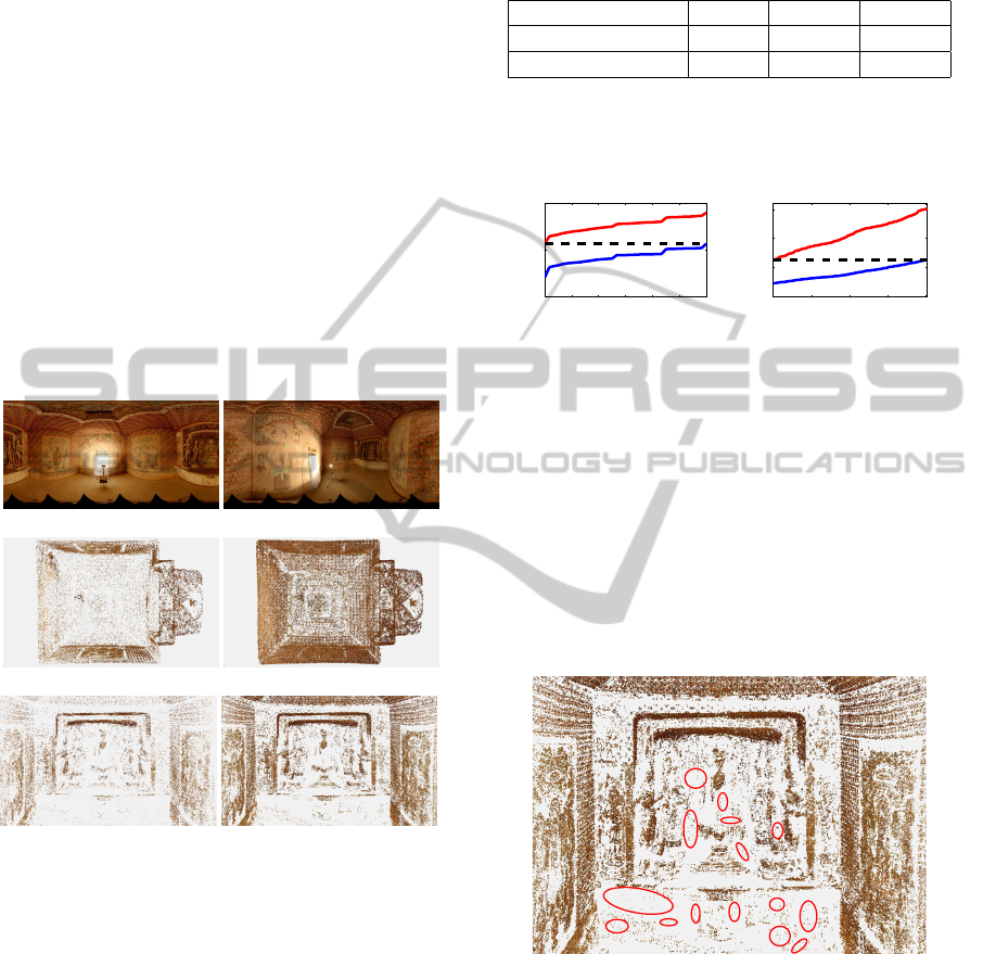
(a) (b)

(e) (f)

Figure 5: (a) and (b): Two images captured in the Mogao

Cave. (c) and (d): Top view of the cave using S

and S

. (e)

and (f): Front view of the statues using S

and S

5.2 Mogao Cave

This dataset consists of 9 images taken inside the Mo-

gao Cave number 322. In total, 36 pairs were used

with 3 layers of features computed for each image.

Table 1 summarizes the approximate number of key-

points detected per layer for each image. The third

layer contains roughly 5 times the number of features

in the ﬁrst layer, i.e. we considerably increased im-

age sampling. Figure 5 shows the results produced

by our algorithm for this dataset. The evolution of

the number of anchor points n is depicted in Figure 6-

(b). The blue curve shows how n raises from S

to S

Table 1: Approximate number of SASIFT keypoints de-

tected per layer for each image. The lables L1, L2 and L3

identify the corresponding layer.

Dataset L1 L2 L3

Mogao Cave 60000 175000 300000

St. Martin Square 84000 510000 -

during the ﬁrst matching step. Accordingly, the red

curve illustrates the behaviour of n during the second

matching step, i.e. from S

to S

0 6 12 18 24 30 36

x 10

Number of pairs

Number of points

(a)

0 40 80 120 160

x 10

Number of pairs

Number of points

(b)

Figure 6: Number of points versus number of image pairs

for the ﬁrst (blue) and second (red) matching steps. (a) Mo-

gao Cave: S

, S

and S

contain 84591, 228044 and 359981

anchor points. (b) Saint Martin Square: S

, S

and S

con-

tain 16627, 57706 and 100179 anchor points.

Figure 7 shows the importance of matching based

on apical angles. In comparison to Figure 5-(f), the

ellipses indicate areas where new points were added.

This result was produced by ﬁrst computing S

, which

delivered 28227 new anchor points, and then applying

the matching based on anchor points one more time,

with τ = 0.90. The ﬁnal number of points is 409744.

Figure 7: Importance of matching based on apical angles.

See text for details.

5.3 Saint Martin Square

The images were taken around a fountain located in

the square. This dataset contains 35 images, lead-

ing to 161 pairs. Here we computed only 2 layers

of features. Figure 8 illustrates the results regarding

the point cloud and Figure 6-(b) shows the evolution

of the total number of anchor points for this dataset.

VISAPP2013-InternationalConferenceonComputerVisionTheoryandApplications

326

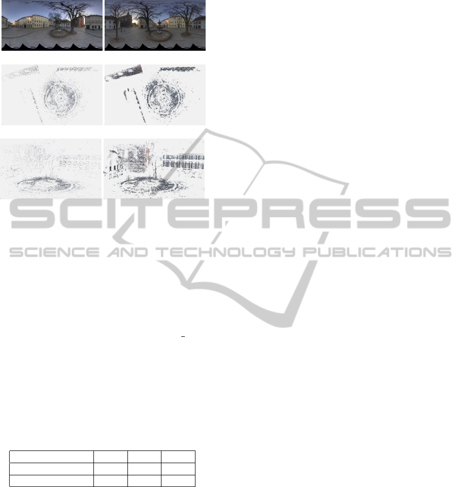
(a) (b)

(e) (f)

Figure 8: (a) and (b): Two exemplary images taken around

the fountain. (c) and (d): Top view of the area using S

and

. (e) and (f): Close-up on the fountain using S

and S

5.4 Reprojection Error

To evaluate the robustness of the proposed approach,

we computed and compared the mean reprojection er-

ror ¯e for S

, S

and S

. The results are summarized

in Table 2. Comparing ¯e(S

) with ¯e(S

), it is clear

that our approach reduces ¯e(S

) to roughly

of its

value. When matching based on apical angles is ap-

plied, it further reduces the mean reprojection error

for the Mogao Cave dataset. This shows that our ap-

proach consistently adds points to the point cloud and

improves the initial scene representation.

Table 2: Mean reprojection error ¯e computed for S

, S

and

, i.e. before and after applying our guided matching tech-

nique. Values are given in pixels.

Dataset ¯e(S

) ¯e(S

)

Mogao Cave 7.51 1.90 1.81

St. Martin Square 4.32 0.97 0.97

6 CONCLUSIONS

This paper presented a method to robustly add 3D

points to sparse point clouds to provide a better repre-

sentation of the underlying scene. We also proposed a

multi-layer feature detection strategy that can be used

with several feature detectors and allows features to

be hierarchically matched. High resolution spherical

images were used as they are more suitable for feature

matching. Moreover, our future work includes the de-

velopment of a dense 3D reconstruction framework

based on this type of images.

ACKNOWLEDGEMENTS

This work was funded partially by the project CAP-

TURE (01IW09001) and partially by the project

DENSITY (01IW12001). The authors would like

to thank Jean-Marc Hengen and Vladimir Hasko for

their technical support.

REFERENCES

Bay, H., Ess, A., Tuytelaars, T., and Van Gool, L. (2008).

Speeded-up robust features (surf). Comput. Vis. Image

Underst., 110(3):346–359.

Furukawa, Y., Curless, B., Seitz, S. M., and Szeliski, R.

(2010). Towards internet-scale multi-view stereo. In

CVPR.

Hiep, V. H., Keriven, R., Labatut, P., and Pons, J.-P.

(2009). Towards high-resolution large-scale multi-

view stereo. In CVPR, pages 1430–1437. IEEE.

Lowe, D. G. (2004). Distinctive image features from scale-

invariant keypoints. International Journal on Com-

puter Vision, 60:91–110.

Lu, X. and Manduchi, R. (2004). Wide baseline feature

matching using the cross-epipolar ordering constraint.

In CVPR, volume 1, pages 16–23, Los Alamitos, CA,

USA. IEEE Computer Society.

N¨oll, T., K¨ohler, J., Reis, G., and Stricker, D. (2012). High

quality and memory efﬁcient representation for image

based 3d reconstructions. In DICTA, Fremantle, Aus-

tralia. IEEE Xplore.

Pagani, A., Gava, C., Cui, Y., Krolla, B., Hengen, J.-M.,

and Stricker, D. (2011). Dense 3d point cloud gener-

ation from multiple high-resolution spherical images.

In VAST, pages 17–24, Prato, Italy.

Pagani, A. and Stricker, D. (2011). Structure from motion

using full spherical panoramic cameras. In OMNIVIS.

Schwartz, C., Weinmann, M., Ruiters, R., and Klein, R.

(2011). Integrated high-quality acquisition of geom-

etry and appearance for cultural heritage. In VAST,

pages 25–32. Eurographics Association.

Tola, E., Lepetit, V., and Fua, P. (2009). Daisy: An efﬁ-

cient dense descriptor applied to wide baseline stereo.

TPAMI, 99(1).

Triggs, B. (2001). Joint Feature Distributions for Image

Correspondence. In ICCV, volume 2, pages 201–208,

Vancouver, Canada. IEEE Computer Society.

RobustGuidedMatchingandMulti-layerFeatureDetectionAppliedtoHighResolutionSphericalImages

327