
Learning and Classification of Car Trajectories
in Road Video by String Kernels
Luc Brun
1
, Alessia Saggese
2
and Mario Vento
2
1
GREYC UMR CNRS 6072 ENSICAEN - Universit
´
e de Caen Basse-Normandie, 14050 Caen, France
2
Dipartimento di Ingegneria Elettronica e Ingegneria Informatica, University of Salerno, I -84084 Fisciano (SA), Italy
Keywords:
Abnormal Trajectories Recognition, Abnormal Behaviors Recognition, String Kernel.
Abstract:
An abnormal behavior of a moving vehicle or a moving person is characterized by an unusual or not expected
trajectory. The definition of expected trajectories refers to supervised learning, where an human operator
should define expected behaviors. Conversely, definition of usual trajectories, requires to learn automatically
the dynamic of a scene in order to extract its typical trajectories. We propose, in this paper, a method able to
identify abnormal behaviors based on a new unsupervised learning algorithm. The original contributions of the
paper lies in the following aspects: first, the evaluation of similarities between trajectories is based on string
kernels. Such kernels allow us to define a kernel-based clustering algorithm in order to obtain groups of similar
trajectories. Finally, identification of abnormal trajectories is performed according to the typical trajectories
characterized during the clustering step. The experimentation, conducted over a real dataset, confirms the
efficiency of the proposed method.
1 INTRODUCTION
In the last decades the significant increase in the num-
ber of available cameras has lead the scientific com-
munity to investigate on control systems able to au-
tomatically generate alarms. Most of researches re-
cently conducted in the field of behavior analysis has
focused on the recognition of simple activities (i.e.
running, waving, jumping) in high resolution videos,
by exploiting the details of human body (Aggarwal
and Ryoo, 2011). The main problem in such an ap-
proach lies in the fact that in a lot of real applica-
tions detailed information related, for instance, to the
pose or to the clothing colors of people are not avail-
able, since objects are in a far-field or video has a
low-resolution: the only information that a video an-
alytic system is reliably able to extract is a noisy tra-
jectory. For these reasons, the moving objects’ tra-
jectories need to be stored (d’Acierno et al., 2012a)
(d’Acierno et al., 2012b) and analyzed, in order to
understand objects’ behaviors, identifying abnormal
ones (Acampora et al., 2012).
The architecture of a system for behavior un-
derstanding is usually based on the following steps:
learning phase and operating phase. The learning
phase aims at extracting prototypes of normal trajec-
tories; it can be performed by following one of these
two models: (Chandola et al., 2009): supervised and
unsupervised. Techniques trained in supervised mode
(Zhou et al., 2007) assume the availability of a train-
ing data set with labeled instances of normal as well as
abnormal trajectories. However, such an approach has
a significant drawback: abnormal instances are usu-
ally far fewer compared to normal ones in the train-
ing set, so implying that the prototypes extracted for
abnormal trajectories are not accurate and represen-
tative. Techniques operating in unsupervised mode
(Morris and Trivedi, 2011) do not require labeled data
since they make the implicit assumption that normal
instances are far more frequent than abnormal ones.
An unsupervised learning phase makes the control
system context-independent and can be easily applied
in different real environments, since it does not use
human knowledge. This is a very important and not
negligible feature, since it allows the system to au-
tonomously understand dynamics within a scene.
In this paper, we propose an unsupervised ap-
proach: an abnormal trajectory refers to something
that the control system has never (or rarely) seen.
However, a system that raises an alarm for each trajec-
tory which has not been seen before risks to generate
too many false alarms: the system needs to identify
a normal trajectory as one enough similar to one or
more trajectories that the system already knows. For
709
Brun L., Saggese A. and Vento M..
Learning and Classification of Car Trajectories in Road Video by String Kernels.
DOI: 10.5220/0004301207090714
In Proceedings of the International Conference on Computer Vision Theory and Applications (VISAPP-2013), pages 709-714
ISBN: 978-989-8565-47-1
Copyright
c
2013 SCITEPRESS (Science and Technology Publications, Lda.)
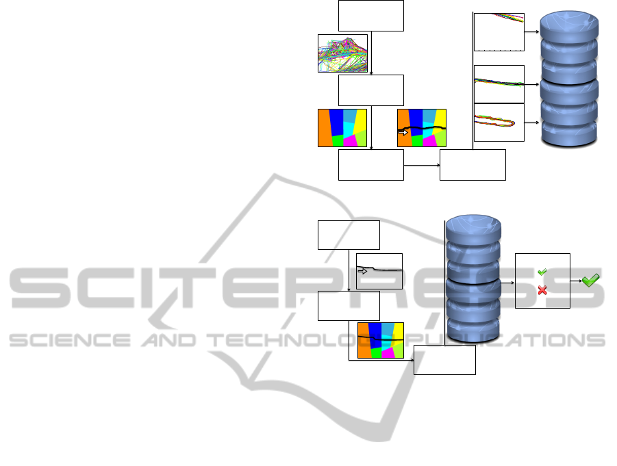
this purpose, we propose a learning phase based on
the following steps, as depicted in Figure 1(a):
Trajectory Extraction: the tracking algorithm de-
tailed in (Di Lascio et al., 2012) is applied in order
to extract moving objects’ trajectories from a video
for a long time period.
Trajectories Representation: the scene is parti-
tioned into zones according to the distribution of tra-
jectories; starting from this, each trajectory is rep-
resented as a sequence of symbols, according to the
zones crossed in the scene.
Trajectories Similarity Computation: similarity
between two trajectories is evaluated by using a
kernel-based method. The main advantage in this
choice lies in the fact that we may combine these
kernels with a large class of clustering and machine
learning algorithms, which can be expressed using
only scalar product between input data.
Clustering: Given the kernel, a novel clustering al-
gorithm is applied in order to extract clusters of tra-
jectories inside the scene. Each cluster encodes a type
of normal trajectories, dynamically extracted from the
scene.
Once extracted the prototypes of normal trajecto-
ries, the control system can start the operating phase,
depicted in Figure 1(b): for each detected abnormal
trajectory, it raises an alarm. In particular we pro-
pose to subdivide the operating phase in the following
steps:
Trajectory Extraction: the trajectory is extracted
from a video by using the tracking algorithm detailed
in (Di Lascio et al., 2012).
Trajectory Representation: the extracted trajectory
is represented as a sequence of symbols.
Classification: the trajectory is compared with the
prototypes of each cluster and a similarity value is ob-
tained for each comparison.
Decision: the computed similarity values are pro-
cessed; if such similarities are sufficiently high the
trajectory is considered normal (3), otherwise it is
considered abnormal (7). In this way, the proposed
system is able to identify both rare and atypical tra-
jectories: the former refer to something that does not
appear in the training set (or only rarely appears);
the latter consider all those trajectories differing in a
slightly but significant way from a group of normal
trajectories.
In this paper we focus on the classification phase.
A brief description of the learning phase will be pro-
vide in Section 2; more details can be found in (Brun
et al., 2012); furthermore, Section 3 shows the ap-
TRAJECTORY)
EXTRACTION)
SCENE)PARTITION)
TRAJECTORY)
REPRESENTATION)
A
B
C
D
E
F
G
H
CLUSTERING)
ABFD
0 50 100 150 200 250 300 350 400 450
0
50
100
150
200
250
300
350
0 50 100 150 200 250 300 350 400 450
0
50
100
150
200
250
300
350
0 50 100 150 200 250 300 350 400 450
0
50
100
150
200
250
300
350
Cluster 1
Cluster 2
Cluster n
…
PROTOTYPES OF
“NORMAL
TRAJECTORIES”
(a)
TRAJECTORY)
EXTRACTION)
TRAJECTORY)
REPRESENTATION)
CLASSIFICATION)
NORMAL/))
)
ABNORMAL))
)
DETECTION)
ABFD
PROTOTYPES OF
“NORMAL
TRAJECTORIES”
(b)
Figure 1: Learning phase (a) and operating phase (b).
proach used to verify if a novel trajectory is normal or
abnormal. Experimental results, which confirm the
efficiency of the proposed method, are finally pre-
sented in Section 4.
2 LEARNING PHASE
A trajectory t can be seen as a sequence of k spatio-
temporal points p
i
= [p
i
x
, p
i
y
, p
i
t
]: t =< p
1
, p
2
,..., p
k
>.
This representation has two main drawbacks: first, a
trajectory results in a very large amount of data to be
managed; second, row data are more sensible to noise
and tracking errors, and thus a filtering of each trajec-
tory is needed before use. Furthermore, if a system
considers the similarity between row data, it can in-
troduce non relevant differences between trajectories.
For example, many trajectories on a garden path may
be considered as similar independently of the exact
position of people on the path.
For this reason, a common representation of a tra-
jectory consists in a reduced sequence of symbols,
namely a string, aiming to preserve only the discrim-
inant information and to reduce the space required to
store trajectories.
The discriminant information to be preserved is
VISAPP2013-InternationalConferenceonComputerVisionTheoryandApplications
710

strongly influenced by the aim of the system: as a
matter of fact, in order to verify, for instance, if a per-
son is moving in the opposite direction of a crowd or if
a vehicle is driving on the emergence line on the high-
way, the most discriminant feature is the sequence of
zones crossed by the moving object. Such scenarios
can be labeled as constrained: the moving objects are
expected to follow given paths within the scene.
Scene Partitioning: first, we need to partition the
scene into a set of zones, hence associating a single
symbol to a sequence of points and eliminating non
discriminant information. A common very simple
strategy is to partition the space using a fixed-size uni-
form grid. The main drawback in such an approach
lies in the fact that each zone has an uneven statis-
tics, causing only a suboptimal statistical segmenta-
tion of trajectories. Furthermore, it is evident that the
distribution of trajectories in the scene highlights re-
gion of interests, in which the major parts of trajec-
tories lie and for which we need an higher level of
detail. In order to overcome these limitations, we con-
sider the adaptive method that we recently proposed
in (Brun et al., 2012), aimed at minimizing the mean
error made when assimilating a trajectory to its zone.
The main idea behind our algorithm is to exploit the
distribution of the training set by taking into account
the density, as in the clustering algorithm proposed in
(Brun and Tr
´
emeau, 2002). As a consequence of this
partitioning criterion, areas in the scene in which most
of trajectories lie are represented with an higher num-
ber of zones. A detailed description of the algorithm
can be found in (Brun et al., 2012).
Trajectory Representation: once partitioned the
scene into zones, a trajectory is segmented into l seg-
ments, being the j−th segment s
j
the sequence of
points lying in the same zone. By means of the op-
erator α(•), each segment is mapped into a symbol
of our alphabet, each symbol identifying the passing
through a zone. Furthermore, information about the
speed and the shape of each segment is evaluated by
the θ(•) operator, thanks to the Bernstein Polynomial
Approximation. Thanks to this representation, each
trajectory can be seen as t = {< α(s
1
),...,α(s
l
) >,<
θ(s
1
),...,θ(s
l
) >}.
Trajectories Similarity: the complexity and the dif-
ferent typology of information to take into account
to represent a trajectory result in a complex strategy
to verify the similarity between trajectories. In fact,
we need to manage a string for the position and a
sequence of numerical values for the speed and the
shape, respectively obtained by means of the α(•) and
the θ(•) operators.
In the last years, a lot of different methods based
on dynamic programming have been proposed in or-
der to evaluate the similarity between two sequences,
ranging from the Smith Waterman algorithm (Saigo
et al., 2004) to the edit-distance (Neuhaus and Bunke,
2006). The main problem lies in the fact that, al-
though these methods are able to compute a similarity
value, they do not define a metric. In order to solve
these problems, we propose a novel similarity metric
based on kernels: the main advantage is that the prob-
lem can then be formulated in an implicit vector space
on which statistical methods for pattern analysis can
be applied. Furthermore, thanks to this choice, it is
possible to evaluate the similarity between sequences
of symbol with different length, so avoiding to force
the representation of trajectories to a vector of fea-
tures with a fixed dimension.
In particular, we construct our kernel starting from
the Fast Global Alignment Kernel (FGAK) proposed
in (Cuturi, 2011). The main idea of all global align-
ment kernels is to measure the similarity between
two sequences by summing up scores obtained from
local alignments with gaps of the sequences. An
alignment between two sequences x = {x
1
,...,x
n
} and
y = {y
1
,...,y
m
} of length n and m respectively is a
pair of increasing integral vectors (π
1
,π
2
) of length
p < n + m, such that 1 = π
1
(1) ≤ ... ≤ π
1
(p) = n
and 1 = π
2
(1) ≤ ... ≤ π
2
(p) = m, with unary incre-
ments and no simultaneous repetitions. Let A(n,m)
be the set of all the possible alignments between the
two time series of lengths n and m. The global align-
ment kernel (GAK) is defined as:
k
GA
(x,y) =
∑
π∈A(n,m)
|π|
∏
i=1
k(x
π
1
(i)
,y
π
2
(i)
). (1)
Starting from the representation of our trajectories,
we need to define the kernel k(.,.) in equation 1 which
combines the different features related to a trajectory.
In particular, we defined the following kernels.
In order to speed up the computation of the kernel,
we use the triangular kernel for integers, also known
as Toeplitz kernel, to compare the symbols x
i
and y
j
:
w(i, j) =
1 −
|i − j|
T
, (2)
where T is the order of the kernel. The main advan-
tage in the use of the triangular kernel is that it allows
to only consider a smaller subset of alignments.
Furthermore, in order to evaluate the similarity
between two strings α(x) and α(y) encoding the se-
quences of zones respectively traversed by trajectories
x and y, we use a dirac kernel δ(α(x
i
),α(y
i
)), defined
as:
δ(α(x
i
),α(y
i
)) =
(
0 if α(x
i
) 6= α(y
i
)
1 if α(x
i
) = α(y
i
)
(3)
LearningandClassificationofCarTrajectoriesinRoadVideobyStringKernels
711

The Dirac Kernel is combined with the Toeplitz Ker-
nel so obtaining:
k
Z
(x
i
,y
j
,i, j) = w(i, j) • δ(α(x
i
),α(y
j
)). (4)
The main lack of this similarity evaluation lies in the
fact that the proximity of two zones is not consid-
ered. In order to overcome this limitation by taking
into account adjacency relationships between zones,
a weighted dirac kernel is also exploited:
k
W Z
(x
i
,y
j
,i, j) = w(i, j) • δ
w
(α(x
i
),α(y
j
)). (5)
Zones are mapped into a non-oriented weighted graph
G = {V,E,w}, whose vertices V = {V
1
,...,V
N
} iden-
tify zones and whose edges E = {E
1
,...,E
L
} identify
proximity of two zones. Each edge is associated to a
weight e
v
1
,v
2
, identifying the number of pixels sepa-
rating two zones.
δ
w
(α(x
i
),α(y
i
)) =
0 if α(x
i
) 6= α(y
i
)
and e
α(x
i
),α(y
i
)
/∈ E
e
I
α(x
i
),α(y
i
)
if e
α(x
i
),α(y
i
)
∈ E
1 if α(x
i
) = α(y
i
)
(6)
where e
I
α(x
i
),α(y
i
)
is a normalized version of e
α(x
i
),α(y
i
)
,
obtained by dividing e
α(x
i
),α(y
i
)
by two times the
length of the longest zone’s border.
Finally, the evaluation of the similarity related to
the velocity and to the shape is based on the follow-
ing speed and shape kernel, used instead of the Gaus-
sian one in order to guarantee the p.d. of k
GA
(Cuturi,
2011):
k
SS
(θ(x
i
),θ(y
i
)) = e
−φ
σ
(θ(x
i
),θ(y
i
))
, (7)
where
φ
σ
(θ(x
i
),θ(y
i
)) =
1
2σ
2
||θ(x
i
) − θ(y
i
)||
2
+
log
2 − e
−
|θ(x
i
)−θ(y
i
)||
2
|
2σ
2
.
(8)
The combination of these two last kernels is de-
fined as:
k
(W )ZSS
(x
i
,y
j
,i, j) =
k
(W )Z
(α(x
i
),α(y
j
)) • k
SS
(θ(x
i
),θ(y
i
)). (9)
Starting from Equation 1, the products of any of the 4
kernels (k
Z
, k
W Z
, k
ZSS
and k
W ZSS
) can be considered
to obtain the final kernel k
GA
. Finally, a normalization
of the kernel is performed in order to normalize ker-
nel’s values in the interval [0,1]. Therefore, the final
normalized kernel k
N
GA
is:
k
N
GA
(x
i
,y
j
,i, j) =
k
GA
(x
i
,y
j
,i, j)
p
k
GA
(x
i
,x
i
,i, i) ∗ k
GA
(y
j
,y
j
, j, j)
.
(10)
Clustering: from a general point of view, the goal
of a clustering algorithm is to find a fixed number
N
C
of groups that are both homogeneous and well
separated, that is, trajectories within the same group
should be similar and entities in different groups dis-
similar. In our context, we aim at exploiting a clus-
tering algorithm in order to obtain a set of prototypes
of normal trajectories. In the last decades, a lot of
graph-based clustering algorithms (Schaeffer, 2007)
(Foggia et al., 2008) have been exploited. Although
these techniques seem to provide good results, they
do not allow to readily verify if a novel trajectory be-
longs to a cluster, that is our main objective. In order
to overcome these limitations, we consider the novel
and efficient kernelized clustering algorithm that we
recently proposed in (Brun et al., 2012) and that we
briefly summarize in the following: the cluster with
the maximum squared error is selected and then split
into two different clusters along the major axis, com-
puted by means of a Kernel PCA (Sch
¨
olkopf et al.,
1998). Since in our context the number of clusters
can not be fixed a priori, we choose to use as stop
condition a lower bound on the mean squared error
made when assimilating one trajectory to its cluster.
In this way, the system does not need knowledge of
the human operator about the environment, but is able
to determine the optimum number of clusters starting
from the distribution of trajectories.
3 OPERATING PHASE
The operating phase aims at identifying abnormal be-
haviors according to the set of typical trajectories de-
termined during the learning phase (Section 2). In
particular, our algorithm evaluates the distance be-
tween a trajectory t
s
and all cluster’s centers C
1
,...C
N
C
obtained during the learning phase. The cluster with
the closest mean from t
s
is selected as the potential
typical trajectory followed by t
s
. An additional test
should then be performed in order to determine if t
s
belongs to this closest cluster. According to this last
test t
s
is classified as normal (it belongs to one cluster
encoding typical trajectories) or an alert is raised and
t
s
is classified as an abnormal behavior.
Classification. Les s denote the string associated to
t
s
and ψ
s
the projection of s into the Hilbert space
encoded by one of our kernel. The squared distance
between ψ
s
and the mean µ
t
of a cluster C
t
is defined
by:
d
2
t
(µ
t
,Ψ
s
) =< µ
t
,µ
t
> + < Ψ
s
,Ψ
s
> −2 < µ
t
,Ψ
s
>
= 1 + 1 − 2 < µ
t
,Ψ
s
>= 2(1− < µ
t
,Ψ
s
>)
= 2
1 −
1
|C
t
|
∑
s
i
∈C
t
k(s, s
i
)
!
. (11)
VISAPP2013-InternationalConferenceonComputerVisionTheoryandApplications
712
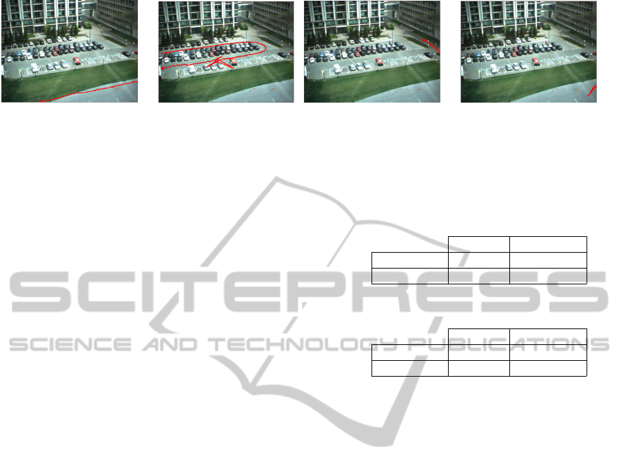
(a) (b) (c) (d)
Figure 2: Abnormal trajectories classified as normal (a) (b) and normal trajectories classified as abnormal (c)(d).
Decision. Let C
∗
t
denote the cluster with the clos-
est center (µ
∗
t
) determined according to equation 11.
Since our clustering algorithm always split clusters
according to their axis of greatest variance, we con-
sider that the covariance matrix of each cluster is ap-
proximately diagonal. In this case, a threshold on
the Gaussian probability that string t
s
belongs to C
∗
t
is approximated by comparing the squared distance
d
2
(µ
∗
t
,Ψ
s
) with a multiple of the squared error of C
∗
t
:
d
2
(µ
∗
t
,Ψ
s
) ≤ α ∗ MSE(C
∗
t
). (12)
Conversely to the parameter ν of one class
SVM (Cortes and Vapnik, 1995), a high value of α
provides a better generalization but may increases the
number of false positive in the test determining the
classification to C
∗
t
.
4 EXPERIMENTAL RESULTS
The proposed method has been validated on the MIT
trajectories dataset (Wang et al., 2011), a standard and
freely available dataset composed by 40.453 trajec-
tories obtained from a parking lot scene within five
days. The experiments have been conducted on a
MacBook Pro equipped with Intel Core 2 Duo run-
ning at 2.4 GHz. Starting from the entire dataset
D, a subset D
∗
of trajectories belonging to vehicles
(10.335) has been manually extracted by an expert
and the proposed system has been evaluated.
The dataset D
∗
has been divided into three folds
and one of these has been used for the learning phase.
The remaining two folds have been mixed with the
remaining trajectories (D \D
∗
) and are used to test the
system. The tests have been performed by computing
the similarity between trajectories by using the Dirac
Kernel and the Weighted Dirac Kernel. The obtained
confusion matrix is reported in Table 1. The results,
for a fixed value of α (α = 2), show that the Weighted
Dirac Kernel provides a better generalization than the
Dirac Kernel, without paying in terms of false positive
errors.
Table 1: Misclassification Matrix obtained by using Dirac
Kernel (a) and Weighted Dirac Kernel (b).
(a)
Predicted Class
Normal Abnormal
GT
Normal 84.10% 21.40%
Abnormal 15.90% 78.60%
(b)
Predicted Class
Normal Abnormal
GT
Normal 85.30% 7.10%
Abnormal 14.70% 92.90%
In any case, starting from the obtained results,
which are sufficiently good for most practical applica-
tions, we can enforce the effectiveness of the method
by drawing some considerations about the nature of
the errors; as we will show in the following, most
of the errors can be considered fake, being strongly
related to ambiguous interpretations of the trajecto-
ries during the manual labeling phase. An example is
shown in Figure 2(a): the trajectory in red is labeled
as abnormal in the ground truth, since it refers to a
vehicle’s trajectory partially located in the grass (or to
an error of the tracking phase as well); our method, as
well as any other kinds of methods based for their na-
ture on shape and position similarities, has no chance
to give a correct answer and classifies such a trajec-
tory as normal, since it is very similar to those normal
which avoid the grass just for a few centimeters. This
error cannot be avoided by any system based on simi-
larity measure, because only the introduction of areas
boundaries could make the system able to provide a
correct answer by boundary cross detection. Similar
situation occurs in Figure 2(b), where the vehicle tries
to park, but because of place lack, leaves out after a
complete turn. In this case, the description of the tra-
jectory follows a regular and normal path, except for
a very limited stretch, reproducing the same typology
of error occurring in the previous case.
Opposite kinds of error occur in Figures 2(c) and
2(d). In this case, the two trajectories are manually
labeled as normal with respect to their semantic, but
LearningandClassificationofCarTrajectoriesinRoadVideobyStringKernels
713

can also refer to tracking errors because of their very
short lengths. The system in such a situations has not
sufficient information and then is not able to reliably
associate the two trajectories to any cluster containing
normal trajectories.
In conclusion the performance, yet acceptable for
many practical application, can be considered even
better at the light of the above considerations. How-
ever, we could think, as future work, the introduc-
tion of a mixed solution based both on clustering and
boundary-constraints so as to catch the advantages of
both these approaches, even at the cost of introduc-
ing a little more heavy a priory knowledge about the
scene to be processed.
5 CONCLUSIONS
We have proposed a system able to identify abnor-
mal trajectories without the explicit definition of the
rules by a human operator. It has been achieved by
introducing an unsupervised method able to deduce
properties of a scene from a set of trajectories. Start-
ing from a set of normal trajectories acquired by a
video analytics system, our method represents each
trajectory by a sequence of symbols associated to rel-
evant features of trajectories (crossed zones, shape
and speed in each zone). This quantization is obtained
by partitioning the scene into a fixed number of adap-
tive zones. Similarity between trajectories is evalu-
ated by means of a fast alignment global kernel. Tra-
jectories are then grouped into homogenous clusters
encoding normal trajectories. The classification into
(ab)normal trajectories is performed by taking advan-
taging on the statistical properties of the clusters. Ex-
periments have been performed on a real dataset and
the obtained results, compared with other state of the
art methods, confirm the efficiency of the proposed
approach.
ACKNOWLEDGEMENTS
This research has been partially supported by
A.I.Tech s.r.l. (a spin-off company of the University
of Salerno, www.aitech-solutions.eu).
REFERENCES
Acampora, G., Foggia, P., Saggese, A., and Vento, M.
(2012). Combining neural networks and fuzzy sys-
tems for human behavior understanding. In Proceed-
ings of the IEEE AVSS Conference, pages 88–93.
Aggarwal, J. and Ryoo, M. (2011). Human activity analy-
sis: A review. ACM Comput. Surv., 43(3):16:1–16:43.
Brun, L., Saggese, A., and Vento, M. (2012). A clustering
algorithm of trajectories for behaviour understanding
based on string kernels. In Proceedings of the 2012
SITIS Conference, pages 267–274. IEEE.
Brun, L. and Tr
´
emeau, A. (2002). Digital Color Imaging
Handbook, chapter 9 : Color quantization, pages 589–
637. Electrical and Applied Signal Processing. CRC
Press.
Chandola, V., Banerjee, A., and Kumar, V. (2009).
Anomaly detection: A survey. ACM Comput. Surv.,
41(3):15:1–15:58.
Cortes, C. and Vapnik, V. (1995). Support-vector networks.
Machine Learning, 20:273–297.
Cuturi, M. (2011). Fast global alignment kernels. In
Getoor, L. and Scheffer, T., editors, Proceedings of
the 28th International Conference on Machine Learn-
ing (ICML-11), ICML ’11, pages 929–936, New York,
NY, USA. ACM.
d’Acierno, A., Leone, M., Saggese, A., and Vento, M.
(2012a). An efficient strategy for spatio-temporal data
indexing and retrieval. In Proceedings of the KDIR
Conference, pages 227,232.
d’Acierno, A., Leone, M., Saggese, A., and Vento, M.
(2012b). A system for storing and retrieving huge
amount of trajectory data, allowing spatio-temporal
dynamic queries. In Proceedings of the IEEE ITS Con-
ference, pages 989,994.
Di Lascio, R., Foggia, P., Saggese, A., and Vento, M.
(2012). Tracking interacting objects in complex sit-
uations by using contextual reasoning. In Csurka,
G. and Braz, J., editors, VISAPP (2), pages 104–113.
SciTePress.
Foggia, P., Percannella, G., Sansone, C., and Vento, M.
(2008). A graph-based algorithm for cluster detection.
IJPRAI, 22(5):843–860.
Morris, B. and Trivedi, M. (2011). Trajectory learning
for activity understanding: Unsupervised, multilevel,
and long-term adaptive approach. Pattern Analy-
sis and Machine Intelligence, IEEE Transactions on,
33(11):2287 –2301.
Neuhaus, M. and Bunke, H. (2006). Edit distance-based
kernel functions for structural pattern classification.
Pattern Recognition, 39(10):1852 – 1863.
Saigo, H., Vert, J.-P., Ueda, N., and Akutsu, T. (2004). Pro-
tein homology detection using string alignment ker-
nels. Bioinformatics, 20(11):1682–1689.
Schaeffer, S. (2007). Graph clustering. Computer Science
Review, 1(1):27–64.
Sch
¨
olkopf, B., Smola, A., and M
¨
uller, K.-R. (1998). Non-
linear component analysis as a kernel eigenvalue prob-
lem. Neural Comput., 10(5):1299–1319.
Wang, X., Ma, K. T., Ng, G.-W., and Grimson, W. E.
(2011). Trajectory analysis and semantic region mod-
eling using nonparametric hierarchical bayesian mod-
els. Int. J. Comput. Vision, 95:287–312.
Zhou, Y., Yan, S., and Huang, T. (2007). Detecting anomaly
in videos from trajectory similarity analysis. In Multi-
media and Expo, 2007 IEEE International Conference
on, pages 1087 –1090.
VISAPP2013-InternationalConferenceonComputerVisionTheoryandApplications
714
