Vehicle Detection with Context

Yang Hu and Larry S. Davis

Institute for Advanced Computer Studies, University of Maryland, 20742 College Park, MD, U.S.A.

Keywords:

Vehicle Detection, Context, Conditional Random Fields, Shadow, Ground, Orientation.

Abstract:

Detecting vehicles in satellite images has a wide range of applications. Existing approaches usually identify

vehicles from their appearance. They typically generate many false positives due to the existence of a large

number of structures that resemble vehicles in the images. In this paper, we explore the use of context infor-

mation to improve vehicle detection performance. In particular, we use shadows and the ground appearance

around vehicles as context clues to validate putative detections. A data driven approach is applied to learn

typical patterns of vehicle shadows and the surrounding “road-like” areas. By observing that vehicles often

appear in parallel groups in urban areas, we also use the orientations of nearby detections as another context

clue. A conditional random ﬁeld (CRF) is employed to systematically model and integrate these different

contextual knowledge. We present results on two sets of images from Google Earth. The proposed method

signiﬁcantly improves the performance of the base appearance based vehicle detector. It also outperforms

another state-of-the-art context model.

1 INTRODUCTION

With the launch of new generation of earth observa-

tion satellites, more and more high-resolution satellite

images with ground sampling distances of less than 1

meter have become publicly available. Small scale

objects such as vehicles can be readily seen in these

images. In this work, we consider the problem of de-

tecting vehicles from such high-resolution aerial and

satellite images. This problem has a number of ap-

plications in trafﬁc monitoring and intelligent trans-

portation systems, urban planning and design, as well

as military and homeland surveillance. In spite of the

increasing resolution of aerial and satellite images,

vehicle detection still remains a difﬁcult problem. In

urban settings especially, the presence of a large num-

ber of rectangular structures brings signiﬁcant chal-

lenges to the detectors.

Vehicle detection has been explored a lot in the

literature. Most approaches only use the appearance

of vehicles for detection. Due to the existence of the

structures that resemble vehicles in the images, these

methods typically generate many false positives. In

this work, we investigate the use of context informa-

tion to improve vehicle detection performance.

Context is a useful information source for vi-

sual recognition. Psychology experiments show that

in the human visual system context plays an im-

port role in recognition (Oliva and Torralba, 2007).

In computer vision, using context has recently re-

ceived signiﬁcant attention. It has been used suc-

cessfully in object detection and recognition (Rabi-

novich et al., 2007; Heitz and Koller, 2008; Divvala

et al., 2009) as well as many other problems such as

scene recognition (Murphy et al., 2003), action clas-

siﬁcation (Marszalek et al., 2009) and recognition of

human-object interactions (Yao and Fei-Fei, 2012).

We explore useful context clues for the detection

of vehicles. The ﬁrst type of context information we

use are shadows. Instead of using image meta-data

to predict the expected location and shape of shad-

ows, we apply a data driven approach to learn the typ-

ical patterns of vehicle shadows from examples. We

also use the ground appearance around a vehicle as

another contextual clue. Unlike previous work (Chel-

lappa et al., 1994; Quint, 1997; Jin and Davis, 2007)

that requires maps of road network registered to im-

agery, we use image appearance and a data driven ap-

proach to determine whether a not a putative vehicle

detection is surrounded by “road-like” pixels. Finally,

by observing that in urban areas vehicles often appear

in parallel groups, we use the orientations of nearby

detections to validate the initial detections. We em-

ploy a conditional random ﬁeld (CRF) to systemat-

ically model and integrate these different contextual

clues. The algorithms are evaluated on two sets of

images from Google Earth. The results indicate that

the proposed context model greatly improves vehi-

715

Hu Y. and S. Davis L..

Vehicle Detection with Context.

DOI: 10.5220/0004302907150722

In Proceedings of the International Conference on Computer Vision Theory and Applications (VISAPP-2013), pages 715-722

ISBN: 978-989-8565-47-1

 2013 SCITEPRESS (Science and Technology Publications, Lda.)

cle detection performance over a baseline appearance

based detector. It also outperforms another recently

proposed context model.

The rest of this paper is organized as follows. We

ﬁrst discuss related work in Section 2. Then, in Sec-

tion 3, we brieﬂy introduce the partial least squares

baseline vehicle detector (Kembhavi et al., 2011) that

we use to obtain the initial detections to build the CRF

model. We present the CRF model, which is used

as a general framework to integrate different context

clues, in Section 4. We then discuss how we model

the three kinds of contextual information, i.e. shadow,

ground and orientations of nearby detections, in Sec-

tion 5. Experiment results are discussed in Section 6.

Finally, we conclude in Section 7.

2 RELATED WORK

Vehicle detection has previously been treated as a

template matching problem, and algorithms that con-

struct templates in 2D as well as 3D have been pro-

posed. Monn et al. (Moon et al., 2002) proposed an

approach to accurately detect 2D shapes and applied it

to vehicle detection. They derived an optimal 1D step

edge operatorand extended it along the boundarycon-

tour of the shape to obtain a shape detector. Choi and

Yang (Choi and Yang, 2009) ﬁrst used a mean-shift

algorithm to extract candidate blobs that exhibit sym-

metry properties of typical vehicles and then veriﬁed

the blobs using a log-polar shape descriptor. Zhao and

Nevatia (Zhao and Nevatia, 2003) posed vehicle de-

tection as a 3D object recognition problem. They used

human knowledge to model the geometry of typical

vehicles. A Bayesian network was used to integrate

the clues including the rectangular shape of the car,

the boundary of the windshield and the outer bound-

ary of the shadow.

The detection of vehicle has also been treated

as a classiﬁcation problem, and different machine

learning algorithms have been exploited for it. Jin

and Davis (Jin and Davis, 2007) used a morpholog-

ical shared-weight neural network to learn an vehi-

cle model. Grabner et al. (Grabner et al., 2008) pro-

posed to use on-line boosting in an interactive train-

ing framework to efﬁciently train and improve a vehi-

cle detector. Kembhavi et al. (Kembhavi et al., 2011)

presented a vehicle detector that improves upon pre-

vious approaches by incorporating a large and rich set

of image descriptors. They used partial least squares,

a classical statistical regression analysis technique, to

project the extremely high-dimensional feature onto a

much lower dimensional subspace for classiﬁcation.

Contextual knowledge has been exploited for ve-

hicle detection in some previous systems. (Chellappa

et al., 1994; Quint, 1997; Jin and Davis, 2007) in-

tegrate external information from site-models or dig-

ital maps to reduce the search for vehicles to cer-

tain image regions such as road networks and parking

lots. Some use a vehicle’s shadow projection as lo-

cal context for vehicles (Hinz and Baumgartner,2001;

Zhao and Nevatia, 2003). In these works, meta-data

for aerial images are used to compute the direction

of sun rays and derive the shadow region projected

on the road surface. Heitz and Koller (Heitz and

Koller, 2008) present a ”things and stuff (TAS)” con-

text model that uses texture regions (e.g., roads, trees

and buildings) to add predictive power to the detec-

tion of objects and applied it to vehicle detection.

3 VEHICLE DETECTION USING

PARTIAL LEAST SQUARES

Our context model is built on the detections from a

sliding window vehicle detector. This detector slides

a window over the image, scores each window ac-

cording to its match to a pre-trained vehicle model,

and returns the windows with locally highest match-

ing scores. The vehicle model can be derived from

most standard classiﬁers. In this work we use a partial

least squares (PLS) based detector (Kembhavi et al.,

2011) to generate the initial detections.

PLS is a method that uses latent variables to

model the relations between sets of observed vari-

ables. The detector ﬁrst uses PLS to project origi-

nal features onto a more compact space of latent vari-

ables. Then quadratic discriminant analysis (QDA)

is applied to classify the windows into vehicle and

background. Although computationally simple, this

detector has been shown to have good detection per-

formance for both vehicles (Kembhavi et al., 2011)

and human (Schwartz et al., 2009).

We use the Histograms of Oriented Gradients

(HOG) (Dalal and Triggs, 2005) feature for the detec-

tor. HOG captures the distribution of edges or gradi-

ents that are typically observed in image patches that

contain vehicles. Each detection window is divided

into square cells and a 9-bin HOG feature is calcu-

lated for each cell. Grids of 2× 2 cells are grouped

into a block, resulting in a 36D feature vector per

block. A multiscale approach that uses blocks at vary-

ing scales and varying aspect rations (1:1, 1:2, and

2:1) is employed (Zhu et al., 2006).

VISAPP2013-InternationalConferenceonComputerVisionTheoryandApplications

716

4 CONTEXT MODEL WITH

CONDITIONAL RANDOM

FIELDS

A detector that only relies on the appearance of the

vehicles will trigger many false alarms at locations

that show similar appearance patterns to vehicles. For

example, in images captured by wide-area motion im-

agery (WAMI) sensors, the vehicle detector is always

confused by electrical units and air conditioning units

on the tops of buildings. We propose to use contextual

information to reduce these false alarms.

One typical source of spatial contextual informa-

tion is shadows. Shadows provide information to dif-

ferentiate physical objects from texture regions with

confusing appearance. The shape of the shadow area

is closely related to the object casting it. These make

shadows important context clue for vehicle detection.

High level scene information is also very useful. Ve-

hicles should always appear on the roads or parking

lots instead of on trees or buildings. Therefore, inves-

tigating the type of the surrounding regions is also a

useful way to validate a detection. Additionally, since

nearby vehicles always move or park in the same ori-

entation, they provide strong contextual support for

each other.

To systematically employ all these sources of in-

formation, we use a conditionalrandom ﬁeld (CRF) to

model and aggregate these contextual cues. After run-

ning the PLS based sliding window vehicle detector,

we construct a graph with the top scoring (and locally

maximal) detections from the detector as nodes and

connect nearby detections (i.e. the distance between

two detections is smaller than a threshold) by an edge.

We then deﬁne a CRF on that graph, which expresses

the log-likelihood of a particular label y (i.e. assign-

ment of vehicle/non-vehicle to each window) given

observed data x as a sum of unary and binary poten-

tials:

−logP(y|x;µ, λ) ∼

∑

, x

)+ (1)

∑

(i, j)∈ε

∑

, y

, x

)

where ε is the set of edges between detections, φ

and

are the unary and pair-wise feature functions re-

spectively, and µ

and λ

are weights controlling the

relative importance of the terms.

Unary potentials measure the afﬁnity of the pix-

els surrounding the detected locations to the presence

of vehicles. The likelihood that a detection window

contains a vehicle according to the PLS based vehicle

detector can be encoded in a unary term:

= 1, x

) = p

(2)

where p

is the conﬁdence score for the ith window

obtained from the detector. The likelihood that the

detected object is accompanied by a vehicle shadow

and the likelihood that the object is on the ground are

also encoded in unary terms.

The binary potentials enforce the consistency of

the labels assigned to neighboring detections accord-

ing to their properties.

In the following sections, we describe the compu-

tation of these potentials in details.

5 CONTEXT CLUES

5.1 Shadow Clue

To use shadows as a context clue, we need to detect

them. Since we are interested in the shadows near

the detected objects, we only detect the shadows in

the areas near the locations obtained from the slid-

ing window vehicle detector. We use the appearance

of local regions to detect shadows. When a region is

in shadow, it becomes darker and less textured (Zhu

et al., 2010). Therefore, the color and texture of a re-

gion can help predict whether it is in shadow. Taking

a rectangular window centered at a detected location,

following (Guo et al., 2011), we ﬁrst segment the win-

dow into regions using the mean shift algorithm (Co-

maniciu and Meer, 2002). Then for each region, the

color and texture are represented with a histogram in

L*a*b space and a histogram of textons respectively.

A SVM classiﬁer with a χ

kernel, which is trained

from manually labeled regions, is used to determine

whether a region is in shadow. After classifying each

region in the window, we obtain a corresponding bi-

nary image which indicates the shadow areas in it.

We use these binary shadow images to compute the

shadow potential in the CRF model.

The absence of shadows in a shadow image can

help to ﬁlter out detections whose appearances are

similar to vehicles but do not have casting shadows.

For detections that have shadows, the position, shape

and size of the shadow area further reveals the type

of the object casting it. In some cases, some image

meta-data may be available, which make it possible

to calculate the shadows using the geometric relation-

ship of the sun and the vehicles. Then we can verify

a detection by comparing this theoretically computed

shadow with the shadow image obtained by running

the shadow detector. In general, however, we do not

have the corresponding meta-data and therefore are

not able to get the theoretical predictions for compar-

ison. In such cases, we learn the characteristics of

typical vehicle shadows from training images.

VehicleDetectionwithContext

717

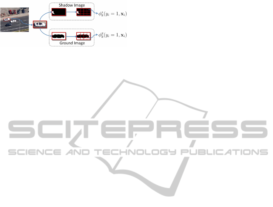
Figure 1: Illustration of the computing of shadow and

ground potentials.

Let I

denote the binary shadow image of the

ith detection; we assume that the likelihood that the

shadow is from a vehicle is linear function of the pix-

els in I

. A set of unary feature functions, each cor-

responding to a pixel in I

is deﬁned, i.e. φ

1, x

) = I

, where I

∈ {0, 1} is the jth pixel in I

Then the coefﬁcients µ

learned by the CRF assign

different weights to the pixels according to their posi-

tions in the window. This deﬁnition, while precisely

differentiating each pixel, greatly increases the com-

plexity of the CRF model. On the other hand, nearby

pixels play similar roles for the prediction. To achieve

a better performance-cost trade off, we can assume

that they share the same weight. Among the many

different potential patterns of sharing the weights, we

simply divide the shadow image into a uniform grid

of cells and have all the pixels in a cell weighted by

the same coefﬁcient. Then the unary potential of the

shadow clue can be expressed as

∑

c(I

)

(3)

where c(I

) indicates the cell pixel I

belongs to.

This is equivalent to

∑

= 1, x

) (4)

where φ

= 1, x

) =

∑

c(I

)=k

. Here we deﬁne a

set of new feature functions, each of which computes

the sum of the pixels in a cell.

Note that the above feature functions are com-

puted over cells, making them robust to some posi-

tion variability of the shadows. This is very impor-

tant since the sliding window vehicle detector usu-

ally moves the windows with step size larger than 1

pixel. It is also not practicable for the detector to con-

sider every orientation. Therefore, the detected vehi-

cle may not lie in the center of the detection window,

and its orientation estimate is subject to some sam-

pling error. By only counting the number of pixels

that are in shadow for each cell, we make the compu-

tation of the shadow potential tolerant to these sources

of variance.

5.2 Ground Clue

Besides shadows, another important contextual clue

for vehicles is they are typically on roads, driveways

or parking lots. To utilize this information, we an-

alyze the surrounding regions of the detected loca-

tions. Speciﬁcally, we consider a rectangle window

centered at a candidate location, segment it into re-

gions and characterize their appearance using color

and texton histograms. Then, the regions are classi-

ﬁed as ground or non-ground by a classiﬁer. A binary

image, which indicates pixels that are classiﬁed as be-

longing to ground, is obtained. We refer to this as the

“ground image” for the candidate location.

The ground potential is calculated in a similar way

as the shadow potential. Let I

denote the ground im-

age of the ith detection. After dividing it into a uni-

form grids of cells, the ground potential is expressed

∑

= 1, x

) (5)

where φ

= 1, x

) =

∑

c(I

)=k

, which corresponds

to the number of pixels that are assigned to ground in

the kth cell.

This method for computing ground potential is

based on a local analysis of the ground. One may

also ﬁrst detect all the ground areas in the entire im-

age and then check the spatial relationships between

the candidate detections and the ground. The TAS

model (Heitz and Koller, 2008) operates in this fash-

ion although the ground areas are detected through

an unsupervised procedure. Since it explicitly con-

siders spatial relationships, it is effective at ﬁltering

out detections that are not near roads. Our method,

on the other hand, not only expects a detection to be

mostly surrounded by ground, but it also can penalize

the situation in which ground appears in the center of

the detection window. This is important for removing

false positives that are on ground but do not contain

vehicles. This crucial difference between two meth-

ods will be illustrated in the experiment results.

5.3 Orientation Clue

In addition to the unary potentials, the frequent co-

occurrence of vehicles can be used to developa binary

potential.

Vehicles, while moving, typically move in the di-

rection of road lanes; in parking, there are also regu-

larities in the patterns of parking. Therefore, nearby

vehicles are usually oriented in the same orientation.

We can use this observation to validate nearby detec-

tions. Speciﬁcally, when two nearby detection win-

dows have the same orientation, it is more probable

VISAPP2013-InternationalConferenceonComputerVisionTheoryandApplications

718

that both of them contain vehicles. On the other hand,

when two nearby detection windows have quite differ-

ent orientations, the probability that they both are true

vehicle windows should be low. Although the speciﬁc

probabilities for different label combinations are hard

to assign manually, they can be estimated from train-

ing data by maximizing the likelihood of the data.

Let d(x

) ∈ (−180, 180] denotes the orientation

of the ith detection window; we classify the orien-

tation relations of two windows into three categories.

In the ﬁrst case, the two windows are in exactly the

same orientation, i.e. |d(x

) − d(x

)| ∈ {0, 180}. In

the second, their orientations are only slightly differ-

ent, i.e. |d(x

) − d(x

)| ∈ (0, d

] ∪ [360 − d

, 360) ∪

[180−d

, 180)∪(180, 180+d

], where d

is a thresh-

old which is set to 20 in experiments. Otherwise, they

are in the third category.

Based on this classiﬁcation, we deﬁne a set of bi-

nary feature functions:

1,···,8

= 0, y

= 0, x

, x

) = [1, a

, a

, 0, 0, 0, 0]

(6)

1,···,8

= 1, y

= 1, x

, x

) = [0, 0, 0, 0, 1, a

, a

]

(7)

1,···,8

= 1, y

= 0, x

, x

) = ψ

1,···,8

= 0, y

= 1,

(8)

, x

) = 0

where



1 if |d(x

) − d(x

)| ∈ {0, 180}

0 otherwise

(9)







1 if |d(x

) − d(x

)| ∈ (0, d

] ∪ [360−d

, 360)

∪[180− d

, 180) ∪ (180, 180+d

]

0 otherwise

(10)







1 if |d(x

) − d(x

)| ∈ (d

, 180−d

)

∪(180+ d

, 360−d

)

0 otherwise

(11)

We cansee that, based on their relativeorientation, the

probabilities that two windows both containing vehi-

cles or not will be different. We also introduce a bias

term, i.e. ψ

= 1, to represent some baseline likeli-

hood that is independent of the orientation clue.

6 EXPERIMENTS

To evaluate the CRF based contextmodel, we perform

experiments on two datasets. Although both of them

are satellite images acquired from Google Earth, the

appearance of the vehicles as well as the surrounding

scenes are quite different in the images of these two

sets.

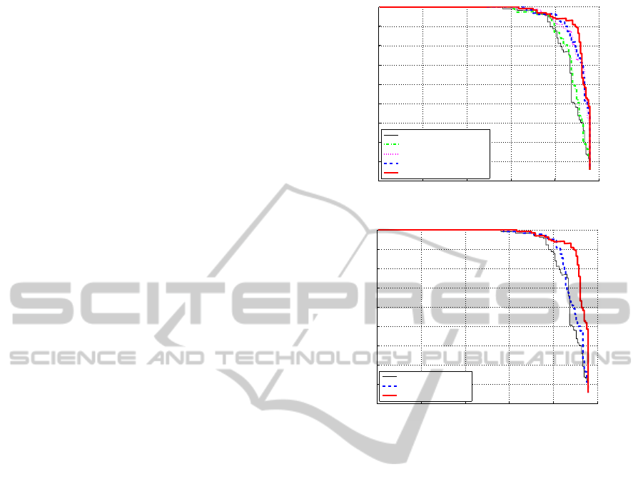
0 0.2 0.4 0.6 0.8 1

0.1

0.2

0.3

0.4

0.5

0.6

0.7

0.8

0.9

Recall

Precision

PLS AP=0.884

CRF(Ori) AP=0.89

CRF(Ori+Sha) AP=0.918

CRF(Ori+Gro) AP=0.92

CRF(Full) AP=0.927

(a) Performance of CRF models with different context clues.

0 0.2 0.4 0.6 0.8 1

0.1

0.2

0.3

0.4

0.5

0.6

0.7

0.8

0.9

Recall

Precision

PLS AP=0.884

TAS AP=0.897

CRF(Full) AP=0.927

(b) Performance comparison with the TAS model.

Figure 2: Precision-recall (PR) curves for Google Earth

Dataset I. AP stands for average precision.

6.1 Google Earth Dataset I

The ﬁrst dataset contains 27 images of an area near

Mountain View, California. There are 391 manu-

ally labeled cars in them. The vehicles are viewed

obliquely with window size of 101× 51 pixels. We

use 14 images to train the CRF model and test the

performance on the remaining 13 images.

We ﬁrst compare the performance of the CRF

models with different context clues. The PLS based

detector (Kembhavi et al., 2011) was used to gener-

ate the initial detections and also serves as the base-

line for comparison. Figure 2(a) shows the precision-

recall curves of CRF with only orientation clue

(CRF(Ori)), with both orientation and shadow clues

(CRF(Ori+Sha)), with both orientation and ground

clues (CRF(Ori+Gro)), and with all of the context

clues (CRF(Full)). The scores from the PLS detec-

tor is included as a unary feature in all these models.

We can see that although the orientation clue alone

only slightly improved the performance, when com-

bined with the shadow clue or the ground clue the de-

tection performance is signiﬁcantly improved. The

effectiveness of shadow and ground clues are similar

VehicleDetectionwithContext

719

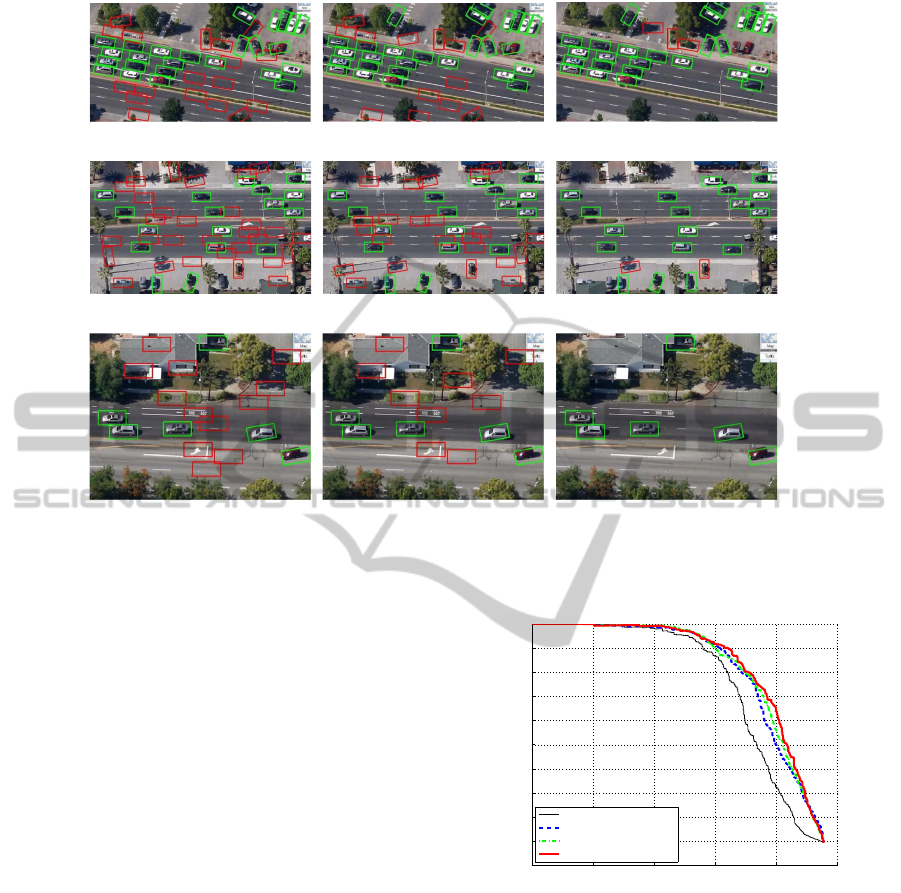
(a) PLS detections (b) TAS detections (c) CRF detections

(d) PLS detections (e) TAS detections (f) CRF detections

(g) PLS detections (h) TAS detections (i) CRF detections

Figure 3: Example images of Google Earth Dataset I, with detections found by the PLS detector, the TAS model and our

CRF(Full) model. The results at recall of 0.9 are shown. Green windows indicate true detections and red windows are false

positives.

and also complementary to each other. When com-

bined together (CRF(Full)), the detection accuracy is

further improved.

We compare the performance of our CRF based

context model with the things and stuff (TAS) context

model (Heitz and Koller, 2008) in Figure 2(b). We

provided the TAS model with the same initial detec-

tions as the CRF model. We can see that although

the TAS model also improved the PLS result, the im-

provement is much smaller than our CRF based con-

text model. This illustrates the advantage of the con-

text clues we used.

We show in Figure 3 some example images, with

detections found by the PLS detector, the TAS model

and our CRF(Full) model respectively at a 90% recall

rate. We can see that the PLS detector generates many

false detections. The TAS model only ﬁlters out some

of the false positives. With our CRF based context

model, most of the false detections are removed.

6.2 Google Earth Dataset II

The second dataset is from TAS (Heitz and Koller,

2008). It contains satellite images of the city and

suburbs of Brussels, Belgium. There are 30 images,

of size 792 × 636 pixels. A total of 1319 cars are

manually labeled in them. A car window is approxi-

0 0.2 0.4 0.6 0.8 1

0.1

0.2

0.3

0.4

0.5

0.6

0.7

0.8

0.9

Recall

Precision

PLS AP=0.738

TAS AP=0.794

CRF(Ori) AP=0.801

CRF(Ori+Gro) AP=0.81

Figure 4: Precision-recall (PR) curves for Google Earth

Dataset II. AP stands for average precision.

mately 45 × 25 pixels. We use half of the images to

train the context models and then test the performance

on the other half of the dataset. The TAS model

was trained with parameters suggested by (Heitz and

Koller, 2008).

We show in Figure 4 the precision-recall curves of

the PLS detector, the TAS model and our CRF based

context models on this dataset. Compared with the

previous dataset, a wider variety of surrounding en-

vironments other than the road occur in the images

in this dataset. This enables the TAS model to better

utilize the stuff, e.g. the roofs of houses, the trees and

VISAPP2013-InternationalConferenceonComputerVisionTheoryandApplications

720

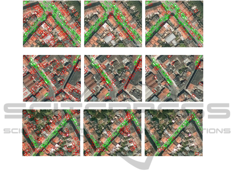
(a) PLS detections (b) TAS detections (c) CRF detections

(d) PLS detections (e) TAS detections (f) CRF detections

(g) PLS detections (h) TAS detections (i) CRF detections

Figure 5: Example images of Google Earth Dataset II, with detections found by the PLS detector, the TAS model and our

CRF(Ori+Gro) model. The results at recall of 0.8 are shown. Green windows indicate true detections and red windows are

false positives.

water regions, to add predictive power to the detection

of vehicles. Therefore, the TAS model achieved much

larger performance improvement over the initial PLS

results on this dataset than on the previous one. On

the other hand, since the vehicles are more spatially

proximate, the CRF model that only uses the orienta-

tion clue also achieved larger performance gain here

than on the other dataset. After adding the ground

clue, the performance was further improved. Since

the sun was overhead, there are hardly any shadows

around the vehicles. We therefore do not have result

using the shadow clue for this dataset.

Figure 5 shows examples of the detections ob-

tained by the three methods. Again we can see the

PLS result includes many false alarms at the 80%

recall point. The TAS model ﬁltered out many of

these false positives, especially those that are not near

roads. The results of our CRF model are even better.

In addition to the windows that are not on the road,

those that are on the road but do not contain vehicles

are also removed.

7 CONCLUSIONS

We explored the use of context information for ve-

hicle detection in high-resolution aerial and satellite

images. We presented an effective way to use both

shadow and ground clues. The consistency of the

orientations of nearby detections was also shown to

be very useful context information. A CRF model

was used to integrate the different types of contextual

knowledge. Experiments on two very different sets

of Google Earth images show that our method greatly

improved the performance of the base vehicle detec-

tor.

ACKNOWLEDGEMENTS

This material is based upon work supported by the

Air Force Research Laboratory (AFRL) under Con-

tract No. FA8750-11-C-0091. Any opinions, ﬁnd-

ings and conclusions or recommendations expressed

VehicleDetectionwithContext

721

in this material are those of the authors and do not

necessarily reﬂect the views of AFRL or the U.S.

Government.

REFERENCES

Chellappa, R., Zheng, Q., Davis, L., Lin, C., Zhang, X., Ro-

driguez, C., Rosenfeld, A., and Moore, T. (1994). Site

model based monitoring of aerial images. In Image

Understanding Workshop.

Choi, J.-Y. and Yang, Y.-K. (2009). Vehicle detection from

aerial images using local shape information. In Pro-

ceedings of the 3rd Paciﬁc Rim Symposium on Ad-

vances in Image and Video Technology.

Comaniciu, D. and Meer, P. (2002). Mean shift: a robust

approach toward feature space analysis. IEEE Trans-

actions on Pattern Analysis and Machine Intelligence,

24(5):603–619.

Dalal, N. and Triggs, B. (2005). Histograms of oriented

gradients for human detection. In Proceedings of the

18th IEEE Conference on Computer Vision and Pat-

tern Recognition.

Divvala, S., Hoiem, D., Hays, J., Efros, A., and Hebert, M.

(2009). An empirical study of context in object detec-

tion. In Proceedings of the 22th IEEE Conference on

Computer Vision and Pattern Recognition.

Grabner, H., Nguyen, T. T., Gruber, B., and Bischof, H.

(2008). On-line boosting-based car detection from

aerial images. ISPRS Journal of Photogrammetry and

Remote Sensing, 63(3):382–396.

Guo, R., Dai, Q., and Hoiem, D. (2011). Single-image

shadow detection and removal using paired regions.

In Proceedings of the 24th IEEE Conference on Com-

puter Vision and Pattern Recognition.

Heitz, G. and Koller, D. (2008). Learning spatial context:

using stuff to ﬁnd things. In Proceedings of the 10th

European Conference on Computer Vision.

Hinz, S. and Baumgartner, A. (2001). Vehicle detec-

tion in aerial images using generic features, group-

ing, and context. In Proceedings of the 23rd DAGM-

Symposium on Pattern Recognition.

Jin, X. and Davis, C. H. (2007). Vehicle detection from

high-resolution satellite imagery using morphologi-

cal shared-weight neural networks. Image and Vision

Computing, 25(9):1422–1431.

Kembhavi, A., Harwood, D., and Davis, L. S. (2011). Vehi-

cle detection using partial least squares. IEEE Trans-

actions on Pattern Analysis and Machine Intelligence,

33(6):1250–1265.

Marszalek, M., Laptev, I., and Schmid, C. (2009). Actions

in context. In Proceedings of the 22th IEEE Confer-

ence on Computer Vision and Pattern Recognition.

Moon, H., Chellappa, R., and Rosenfeld, A. (2002). Opti-

mal edge-based shape detection. IEEE Transactions

on In Image Processing, 11(11):1209–1227.

Murphy, K., Torralba, A., and Freeman, W. (2003). Using

the forest to see the trees: a graphical model relating

features, objects, and scenes. In Advances in Neural

Information Processing Systems.

Oliva, A. and Torralba, A. (2007). The role of context

in object recognition. Trends in Cognitive Sciences,

11(12):520–527.

Quint, F. (1997). MOSES: a structural approach to aerial

image understanding. Automatic Extraction of Man-

made Objects from Aerial and Space Images (II),

pages 323–332.

Rabinovich, A., Vedaldi, A., Galleguillos, C., Wiewiora, E.,

and Belongie, S. (2007). Objects in context. In Pro-

ceedings of the International Conference on Computer

Vision.

Schwartz, W. R., Kembhavi, A., Harwood, D., and Davis,

L. S. (2009). Human detection using partial least

squares analysis. In Proceedings of the 12th Inter-

national Conference on Computer Vision.

Yao, B. and Fei-Fei, L. (2012). Recognizing human-object

interactions in still images by modeling the mutual

context of objects and human poses. IEEE Transac-

tions on Pattern Analysis and Machine Intelligence.

Zhao, T. and Nevatia, R. (2003). Car detection in low res-

olution aerial images. Image and Vision Computing,

21(8):693–703.

Zhu, J., Samuel, K. G. G., Masood, S. Z., and Tappen, M. F.

(2010). Learning to recognize shadows in monochro-

matic natural images. In Proceedings of the 23th IEEE

Conference on Computer Vision and Pattern Recogni-

tion.

Zhu, Q., Avidan, S., Yeh, M.-C., and Cheng, K.-T. (2006).

Fast human detection using a cascade of histograms of

oriented gradients. In Proceedings of the 19th IEEE

Conference on Computer Vision and Pattern Recogni-

tion.

VISAPP2013-InternationalConferenceonComputerVisionTheoryandApplications

722