Contour-based Shape Recognition using Perceptual Turning Points
Loke Kar Seng
Monash University Sunway Campus, Bandar Sunway, Malaysia
Keywords: Shape Recognition, Turning Points, Contour Extraction.
Abstract: This paper presents a new biological and psychologically motivated edge contour feature that could be used
for shaped based object recognition. Our experiments indicate that this new feature perform as well or better
than existing methods. This method have the advantage that computation is comparatively is simpler.
1 INTRODUCTION
Recent works in computer based image recognition
using image-based patches have been very
successful. However there are limitations with this
approach. Some objects are not efficiently
recognized using image patches, as there are some
objects that are more easily categorized by their
shape or contours. The choice of the shape feature is
critical, and ideally the chosen feature should be
used to inform the object contour segmentation.
2 RELATED WORKS
Due to space constraints we discuss some selected
related works. Opelt et al. (2006) used edge
boundary fragments that are specifically selected
from the training procedure that matched edge
chains and centroids in the positive images more
often than negative images. It used a boosting
algorithm to create the detector. Shotton et al. (2008)
also used boundary fragments and calculated the
chamfer distance to find the best match curve. The
Shape Band approach (Bai et al., 2009) used a
coarse-to-fine procedure for object contour
detection. The Shape Band defines a radius distance
from the image sampled edge points from which
approximate directional matching of points could be
performed. Edges within the Shape Band would be
then matched more accurately using Shape Context
(Belongie et al., 2002). Ferrari and colleagues
(Ferrari et al., 2010) used a local feature they called
pairs of adjacent segments (PAS). A codebook is
used for matching object shapes.
These approaches are very similar to our work,
in that edge fragments are used for matching.
However, the features from the curve fragments are
selected without experimental psychological
support. They seemed to be selected based on
training discrimination tests. Features that are
selected based on training tests are probably too
limited because of their dependency on training
examples. In contrast to the works above, our
approach is to select features that have
psychological, perceptual and neurophysiological
basis, i.e. we will make use of the curve’s
perceptually salient point, the turning angle, as the
representation of the curve fragment.
3 PHYSIOLOGICAL AND
PSYCHOLOGICAL EVIDENCE
Research in V4 of the cortex has found that the cells
respond to boundary conformation at a specific
location in the stimulus, such as a certain curvature,
with other parts of the shape having no effect. The
cells appeared to be tuned to curvature and position
within their receptive fields (Pasupathy and Conner,
2001). The findings suggest that at this intermediate
stage, complex objects are represented in parts as
curvature position of their contour components and
not the global shape.
Experiments at the perceptual level indicate that
humans are indeed sensitive to curvatures in
contours. Research has shown that in visual search
task, curved contours pop-out instantly when placed
among distractors of straight contours. In the
experiments by Kristjasson and Tse (2001), it was
487
Seng L..
Contour-based Shape Recognition using Perceptual Turning Points.
DOI: 10.5220/0004304804870491
In Proceedings of the International Conference on Computer Vision Theory and Applications (VISAPP-2013), pages 487-491
ISBN: 978-989-8565-47-1
Copyright
c
2013 SCITEPRESS (Science and Technology Publications, Lda.)

concluded that the visual system is highly sensitive
to curvature discontinuities and not to the rate of
change of curvature. They define curvature
discontinuity as the point where the second
derivative along an image contour is not defined or
where the curvature changes abruptly. In addition,
they found that curvature discontinuities need not be
visible, but can be implied. They reasoned that this
sensitivity is because the curvature discontinuities
are particularly informative about the world
structure.
Attneave (1954) has proposed that information is
concentrated in regions of high curvature of any
object contour. The points along the contour where
curvature reaches (curvature extrema) a local
maximum contains the most information about the
contour. However, not all curvature extrema points
are equally salient. Hoffman and Singh (1997)
proposed that the change of the normal angle from
the two sides of a curve, called the turning angle, as
a determinant of saliency. De Winter and Wageman
(2008) concluded that the turning angle between the
two flanking lines on both side of the curve (Figure
1) is an important factor for perceptual saliency, and
more so than the local curvature. The best
correlations to perceptual saliency are when the
normal is taken from the lines formed by
neighbouring salient points. The strength of saliency
correlates with the sharpness of the turning angle.
Summarizing, it can be concluded that not all
salient points are situated at strong curvature
extrema because some salient points do not occur at
peaks of curvature. The strongest factor underlying
perceptual saliency is the turning angle when it is
measured as the difference in normal of the
adjoining lines between neighbouring salient points.
Saliency correlates to the sharpness of the angle. The
results from these tests provide valuable insights for
building artificial systems.
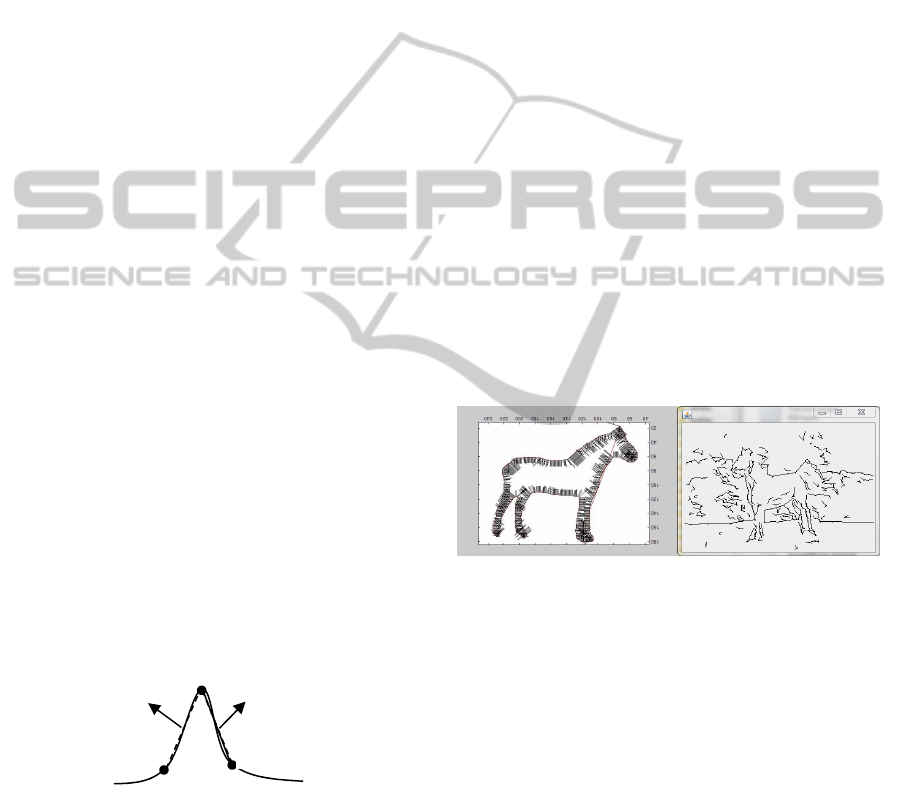
Figure 1: Turning point from normals N
i
and N
i+1
of
salient points.
3.1 Turning Points
The mathematical framework for obtaining points
with high turning angle is based on Feldman and
Singh (2005).
log
(1)
The quantity u() is called the surprisal of which
is the negative log of the probability of .
The surprisal for a curvature (as change in
tangent direction along the curve) using the von
Mises distribution is (Feldman & Singh, 2005) given
as:
∆
cos
∆
(2)
In other words
is proportional to cos
∆
,
and increase monotonically with the scale invariant
version of the curvature ∆:
∝cos
∆
(3)
We disregarded the sign (De Winter & Wageman,
2008) since it does not agree with psychological
experiments. Based on the location of the surprisal,
we calculate the location of the turning angles using
the local neighbourhood peaks of the surprisal
(Figure 2, left). Then the normal angles adjoining
two points on either side of a central point are
calculated (Figure 1). The largest of difference of the
normals within the neighbourhood are kept as a
turning point. All other edge information is
discarded. If we connect all the turning points with a
straight edge then we obtain the result in Figure 2
(right).
Figure 2: Left: Surprisal location and magnitude (as
length). Right: Edges represented by turning points
connected via straight lines.
4 OUR APPROACH
Our basic approach uses turning points (TPs) as
representation of contour fragments. The TPs are
matched against an exemplar using sliding windows
to account for size and location.
The image is pre-processed first by a slight
blurring. The edges are extracted using the Canny
edge detector with all branching and loops removed.
The surprisal is calculated to obtain the TPs.
To obtain the TPs, we first find the local
neighbourhood peaks of the surprisal and measure
the normal angles adjoining two points on either side
of the central point (Figure 1). The peak surprisal
T
i
T
i-1
T
i+1
N
i+1
N
i
VISAPP2013-InternationalConferenceonComputerVisionTheoryandApplications
488

within a window that exceeds a certain threshold is
marked as our TPs.
For every point ̅
in an edge, where the previous
point is ̅
and the next point is ̅
we calculate the
magnitude of the angle formed by the previous
and next point. In practise we take the smoothed
version by averaging over the resolution size of ∆.
̅
∙
̅
̅
∙
̅
(4)
Next we calculate the surprisal
log
expcos
2∆
2
1
(5)
Over a small local neighbourhood, we mark the peak
surprisal with local turning angle that exceeds a
threshold within that window. If there are many
equal maximum values, we pick the one point in the
middle of the window; these will be our turning
points.
From these we obtain the following features
(Figure 3):
,the angle of the TP T
i
to previous T
i-1
and
next turning point, T
i+1
The length and direction of the line
connecting T
i
to the previous T
i-1
and next
turning point T
i+1
.
Feature matching is performed using sliding window
of difference sizes across the image. Across all
windows, the TP at each location are matched with
the exemplar TPs. An edge fragment is successfully
matched if all its turning point features are matched
within a threshold.
Figure 3. Matching of two curves using turning points.
The algorithm returns the bounding box L, of
window size S, where the matching is the maximum,
ie. where the total number of TP matched is at the
maximum.
argmax
,
(6)
T
’
(i) is the i
th
turning point from the sequence of
turning points from the exemplar. T(j) is the j
th
TP
from the sequence of TPs from the test image. L
S
is
the location of the window of size S. The matching
process only considers a TP that is a fixed r distance
from another TP (see Figure 3). T
LS
refers to the TPs
at location L for window of size S. The exemplar,
T’, has a fixed window and size therefore its
location and size is a constant of l
s
.
The detection process requires matching all the
TPs from the same contiguous curve:
,
,
,
,
(7)
,
1
1
1
1
1
1
,
1
,
1
,
1
0
(8)
The function frag(T,i) returns the i
th
TP of the curve
fragment that T belongs to. The current TP T, is
indexed as i and the previous point is i-1 and the
following point is i+1. D
feat
returns a match (value of
1) when the angles of the three consecutive points
T(i-1), T(i) and T(i+1) have approximately the same
turning angles. For point i this is given by
. The
parameters and are fixed constants. D
e
is the
Euclidean distance between the two points, and
ensures that consecutive points are not too far apart.
The window location with the largest match
count is the probable location of the target object.
From the bounding box we obtain these attributes
for classification: centre of gravity of all TPs,
bounding box area, average angular error, total
length matched and number of matched TP.
Attributes calculated from this window are
forwarded to a classification algorithm to determine
if the target object is in the scene image.
5 RESULTS
We use the Weizmann Horse database since
segmented contour outlines are available. For testing
against other categories we use the Broderbund
ClickArt collection, and used scene images of
buildings and wildlife for testing. We tested various
classification algorithms (with best results from
ADTree) using the open source Weka application.
The test was conducted using 10-fold cross
validation averaged 97% correct classification.
Table 1 and Figure 4 show some of the results from
the recognition algorithm.
T
i
T
’
i
T
i-1
T
i+1
T’
i+1
T
Radius r
Contour-basedShapeRecognitionusingPerceptualTurningPoints
489

6 DISCUSSION
There are other works that used turning angles for
contour recognition e.g. (Rusinal et al., 2007;
Kpalma et al., 2008), but those works either tested
on simple images or used turning angles which are
based on technical or mathematical arguments,
whereas our work are derived from psychological
and physiological research.
This work is closest with Shotton et al. (2008)
work, and their results are so far the best, but
compared to Shotton et al., our method achieved
comparable results on the same Weizmann Horse
database. Both approaches work well, despite the
rather challenging images with background clutter;
and wide variety of poses and sizes. The images that
are misclassified are due to significant pose
differences, the small size of the target object and
similarity of the background edges to the training
model edges.
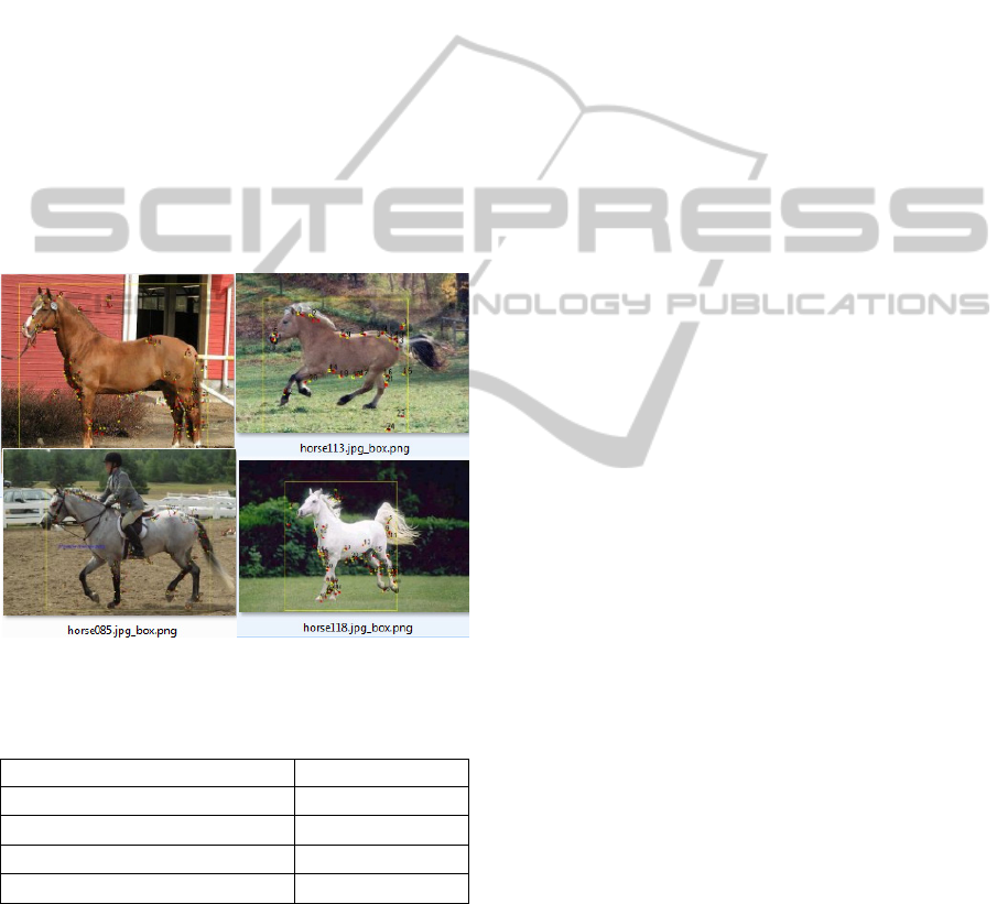
Figure 4: Results of Horse recognition with automatically
detected bounding box (yellow).
Table 1: Comparison of classification results.
Results ROC AUC
Shotton-Boosted Edge 0.9518
Shotton (retrained)-Canny 0.9400
SVM-SIFT 0.8468
Our method 0.9966
Shotton et al., (2008) use a total 228 horse images
and Caltech 101 background set for tests, whereas
we use 238 horse images (from the same Weizman
database) against 244 animals and buildings images
from the Broderbund 65,000 ClickArt collection.
The Caltech 101 background category consist of
assorted scenes around the Caltech campus is
comparable to the building images that we use. The
animal category that we use is likely to be more
challenging and not used in Shotton et al. Based on
the published results (Table 1), our method achieved
a better classification rate.
Our method do not require building a codebook
of contours, as we used turning points that made
comparison easier as we are comparing points with
points, wherease Shotton et al. (2008) used a
comparatively more complicated chamfer distance
measure that required the contour need to be aligned,
complicating the procedure.
In summary, we have presented a perceptually
justified edge boundary feature based on psychology
and neurophysiological research.
REFERENCES
F. Attneave, 1954. "Some informational aspects of visual
perception," Psychological Review, vol. 61, pp. 183-
193.
X. Bai, Q. Li, L. J. Latecki, and W. Liu, 2009. "Shape
band: A deformable object detection approach," in
IEEE Computer Society Conference on Computer
Vision and Pattern Recognition, Miami, Florida, pp.
1335-1342.
S. Belongie, J. Malik, and J. Puzhicha, 2002. Shape
Matching and Object Recognition Using Shape
Contexts," IEEE Transactions of Pattern Analysis and
Machine Intelligence, vol. 24, pp. 509-522.
J. Feldman and M. Singh, 2005. "Information Along
Contours and Object Boundaries," psychological
Review, vol. 112, pp. 263-252.
V. Ferrari, F. Jurie, and C. Schmid, 2010. "From Images to
Shape Models for Object Detection," International
Journal in Computer Vision, vol. 87.
D. D. Hoffman and M. Singh, 1997. "Salience of visual
parts.," Cognition, vol. 63, pp. 29-78.
K. Kpalma, M. Yang, and J. Ronsin, 2008. "Planar Shapes
Descriptors Based on the Turning Angle Scalogram,"
in ICIAR '08 Proceedings of the 5th international
conference on Image Analysis and Recognition, pp.
547-556.
A. Kristjansson and P. U. Tse, 2001. "Curvature
discontinuities are cues for rapid shape analysis,"
Perception & Psychophysics, vol. 3, pp. 390-403.
A. Opelt, A. Pinz, and A. Zisserman, 2006. "A Boundary-
Fragment Model for Object Detection.," in European
Conference on Computer Vision, pp. 575-588.
A. Pasupathy and C. E. Connor, 2001. "Shape
representation in area V4: Position-specific tuning for
boundary conformation," The Journal of
Neurophysiology, vol. 86, pp. 2505-2519.
M. Rusinol, P. Dosch, and J. Llados, 2007. "Boundary
Shape Recognition Using Accumulated Length and
Angle Information," Lecture Notes in Computer
Science, vol. 4478, pp. 210-217.
J. Shotton, A. Blake, and R. Cipolla, 2008. "Multi-Scale
VISAPP2013-InternationalConferenceonComputerVisionTheoryandApplications
490

Categorical Object Recognition Using Contour
Fragments," IEEE Transactions of Pattern Analysis
and Machine Intelligence.
J. D. Winter and J. Wagemans, 2008. "Perceptual saliency
of points along the contour of everyday objects: A
large-scale study," Perception & Psychophysics, vol.
1, pp. 50-64.
Contour-basedShapeRecognitionusingPerceptualTurningPoints
491
