A 3D Segmentation Algorithm for Ellipsoidal Shapes
Application to Nuclei Extraction
Emmanuel Soubies
1
, Pierre Weiss
1
and Xavier Descombes
2
1
ITAV-UMS3039, Universit
´
e de Toulouse, CNRS, Toulouse, France
2
MORPHEME team, INRIA/I3S/iBB, Sophia-Antipolis, France
Keywords:
Nuclei Segmentation, 2D and 3D Images, Graph-cuts, Marked Point Processes, Ellipses and Ellipsoids,
Multiple Object Detection, Multiple Birth and Cut, Bio-imaging.
Abstract:
We propose some improvements of the Multiple Birth and Cut algorithm (MBC) in order to extract nuclei in
2D and 3D images. This algorithm based on marked point processes was proposed recently in (Gamal Eldin
et al., 2012). We introduce a new contrast invariant energy that is robust to degradations encountered in
fluorescence microscopy (e.g. local radiometry attenuations). Another contribution of this paper is a fast
algorithm to determine whether two ellipses (2D) or ellipsoids (3D) intersect. Finally, we propose a new
heuristic that strongly improves the convergence rates. The algorithm alternates between two birth steps. The
first one consists in generating objects uniformly at random and the second one consists in perturbing the
current configuration locally. Performance of this modified birth step is evaluated and examples on various
image types show the wide applicability of the method in the field of bio-imaging.
1 INTRODUCTION
Cell or nuclei segmentation in 2D and 3D is a ma-
jor challenge in bio-medical imaging. New micro-
scopes provide images at higher resolutions, deeper
into biological tissues, leading to an increasing need
for automatic cell delineation. This task may be easy
in certain imaging modalities where images are well
resolved and contrasted, but it remains mostly unre-
solved in emerging fluorescent microscopes dedicated
to live imaging such as confocal, bi-photon, or selec-
tive plane illumination microscopes. These modali-
ties suffer from multiple degradations such as light
attenuation in the sample, heavy noise and spatially
varying blur that make the segmentation task hard
even for human experts.
Our aim in this work is to propose a segmenta-
tion algorithm robust to such situations. Since images
are heavily deteriorated, standard methods aiming at
finding contours based on a sole regularity assump-
tion such as active contours or Mumford-Shah deriva-
tives fail for the segmentation. This observation led
us to introduce strong shape priors: cells are modelled
as ellipses or ellipsoids that should fit the image con-
tents. Unfortunately, adding geometrical constraints
makes the optimization problems highly non convex
and appeal for the development of new global opti-
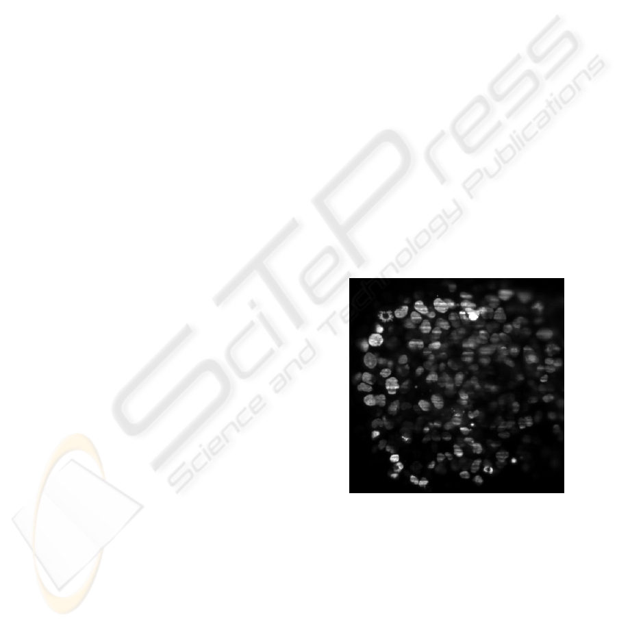
Figure 1: Example of a SPIM image (Multicellular tumor
spheroid).
mization methods.
Following recent works (Descombes et al., 2009;
Descombes, 2011; Gamal Eldin et al., 2012), we use
randomized algorithms that allow to escape from lo-
cal minima. These algorithms are based on marked
point processes. The Marked Point Process (MPP)
approach (Baddeley and Van Lieshout, 1993; Dong
and Acton, 2007) consists in estimating a configura-
tion of geometric objects (in our case ellipses or el-
lipsoids) whose number, location and shape are un-
97
Soubies E., Weiss P. and Descombes X. (2013).
A 3D Segmentation Algorithm for Ellipsoidal Shapes - Application to Nuclei Extraction.
In Proceedings of the 2nd International Conference on Pattern Recognition Applications and Methods, pages 97-105
DOI: 10.5220/0004308100970105
Copyright
c
SciTePress
known. It has proved to be very efficient in numer-
ous image analysis applications as it allows the com-
bination of radiometric information with strong geo-
metrics constraints on the objects but also at a global
scale. Defined by a density against the Poisson pro-
cess measure, its main advantage is to consider a ran-
dom number of objects and can be considered as an
extension of the Markov Random Field approach. A
review of this approach and its applications can be
found in (Descombes, 2011).
The objects are defined on a state space χ = I ×M
by their location and their marks (i.e. geometric at-
tributes). The associated marked point process X is a
random variable whose realisations are random con-
figurations of objects. Considering a Gibbs process,
the modeling consists of an energy construction. Sim-
ilarly to the Bayesian framework, this energy can be
written as the sum of a data term and a prior. In
this paper we consider a pairwise interactions prior
that forbids intersections between objects. Once the
model defined, the solution is obtained by minimiz-
ing the energy. This energy being highly non-convex
requires stochastic dynamics, such as MCMC meth-
ods, to be minimized. The Reversible Jump MCMC
embeded in a simulated annealing framework is a
natural candidate for this task (Green, 1995). How-
ever, in case of simple constraints such as non over-
lap, the recently proposed multiple birth and death al-
gorithm is preferable (Descombes et al., 2009). To
avoid the fastidious calibration of annealing parame-
ters, we propose to revisit the combination of the mul-
tipe births principle with the graph cut paradigm pro-
posed by (Gamal Eldin et al., 2012).
The paper is organized as follows. We formalize
the segmentation problem as a minimization problem
in section 2. Section 3 begins by a global algorithm
description and is followed by a precise description of
each algorithm step. We finish by presenting numeri-
cal results in section 4.
2 PROBLEM STATEMENT
Figure [1] contains typical examples of images en-
countered in biology. It is readily seen from these
images that most nuclei contours can be well approx-
imated by ellipses or ellipsoids, at least at a coarse
scale. Moreover these nuclei cannot overlap due to
obvious physical considerations. We thus formulate
our segmentation problem as that of finding a set of
non overlapping ellipsoids that fit the image contents.
We formalize this statement in the latter.
Let C
n
, n ∈N denote the set of configurations con-
taining n objects that do not overlap. An element
x ∈ C
n
is a set of n non overlapping objects. Since
the number of nuclei in the configuration is unknown,
we aim both at finding this number n
∗
and the best
configuration x ∈ C
n
∗
with respect to a certain data fi-
delity term f (x). Our optimization problem can thus
be formulated as follows. Let
g(n) = min
x∈C
n
f (x)
denote the minimum value of f in the set C
n
. We wish
to find both
n
∗
= argmin
n∈N
g(n)
and
x
∗
= argmin
x∈C
n
∗
f (x).
By convention, we assume that C
0
=
/
0 and that
min
x∈C
0
f (x) = 0. The data term f should thus be neg-
ative for configurations that are likely to represent the
nuclei parameters and positive otherwise. We detail
how the ellipses are parametrized and the construc-
tion of such a function in the following paragraphs.
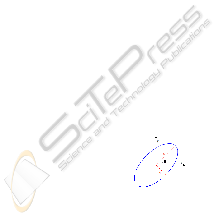
Object Modelling. In 2 dimensions, ellipses are pa-
rameterized using 5 parameters (see Figure 2):
• (x, y) ∈ Ω: center coordinates which should be-
long to the image domain Ω.
• θ ∈ [0,2π[: angle with the horizontal direction.
• 0 < λ
−
< b < a < λ
+
: describe the ellipses minor
and major axes size. λ
−
and λ
+
are user defined
parameters that describe the nuclei maximal size
and ellipticy.
Figure 2: Parameters of the ellipse.
In 3 dimensions, nuclei are parameterized using 9
parameters:
• (x, y,z) ∈ Ω: center coordinates.
• φ, θ, ψ ∈ [0, 2π[
3
: Euler angles to define the ellip-
soids orientations.
• 0 < λ
−
< c < b < a < λ
+
: axes lengths.
ICPRAM2013-InternationalConferenceonPatternRecognitionApplicationsandMethods
98

Overall, it can be seen that objects belong to a
state space χ defined as a parallelepiped:
χ = Ω ×[0,2π[×[λ
−
,λ
+
]
2
(1)
in 2D and
χ = Ω ×[0,2π[
3
×[λ
−
,λ
+
]
3
(2)
in 3D.
In this paper, the objects are denoted ω and their
boundary is denoted ∂ω.
Data Term. Let u : Ω → R denote a grayscale im-
age. In order to define the data term f (x), we asso-
ciate an elementary energy U
d
(ω,u) to each element
ω ∈ x and set:
f (x) =
∑
ω∈x
U
d
(ω,u). (3)
The function U
d
(ω,u) ∈ [−1,1] should be negative if
the object ω is well positioned on the image and pos-
itive otherwise.
In fluorescence microscopy, nuclei are usually
characterized by bright region surrounded by a dark
background since they are stained or genetically mod-
ified in order to express a fluorescent protein. Unfor-
tunately, their radiometry is not constant due to local
bleaching or light attenuation in the deepest layers.
We thus need to construct an energy that is contrast
invariant, meaning that local modifications of the ra-
diometry shall not affect the energy. Such an energy
can be constructed easily by considering the normal to
the image level lines
∇u
|∇u|
where ∇u denotes the usual
gradient in R
d
and |∇u| denotes the gradient magni-
tude in the standard Euclidean norm. This tool is well
known to be contrast invariant. Let us define an en-
ergy U for a given object ω as:
U(ω) =
1
|∂ω|
Z
∂ω
h
∇u(x)
p
|∇u(x)|
2
+ ε
2
,n(x)idx (4)
where h·,·i denotes the standard scalar product, |∂ω|
denotes the length of the object boundary, n(x) de-
notes the outward normal to ω at location x ∈ ∂ω and
ε is a regularization parameter that discard faint tran-
sitions. The behavior of this energy is illustrated on
Fig. 3. Overall, it does what is expected, but as can
be seen on the illustration b) and d) in Fig. 3, badly
located ellipses might have a negative energy and be
kept in the final configuration. It is thus necessary
to modify U in order to promote well located objects
only. A simple way to do so consists in setting:
U
d
(ω,u) = ψ(U(ω),s)
where s ∈] −1, 0] is an acceptance threshold for the
objects. and
ψ(α,s) = min(
1
s + 1
α −
s
s + 1
,1).
Figure 3
.
Figure 4: Graph of the function ψ(α, s) with respect to α
for s = −0.5. Note that the function becomes positive for
values of α > s.
This function is illustrated on Figure 4
Other data terms based on the contrast between
the object interior and the background as presented
by (Gamal Eldin et al., 2012) (in dimension 2) could
also be used but present two drawbacks: first they re-
quire to compute an integral over the interior of the
domain while the proposed approach consist in com-
puting a boundary integral which is faster. Second,
such measures might be inaccurate in the case of very
dense media, where the background can be difficult
to extract. Finally our measure is contrast invariant,
which is central for the targeted applications.
3 MULTIPLE BIRTH AND CUT
ALGORITHM (MBC)
The Multiple Birth and Cut algorithm (MBC) has
been proposed by (Gamal Eldin et al., 2012) for
counting flamingos in a colony. In this section, we
describe the different steps of the MBC algorithm (Al-
gorithm 1).
The main idea consists in generating two random
configurations of non-overlapping objects x and x
0
(birth step) and then keep the subset of objects in
x ∪x
0
that minimizes f (cut step). This process is it-
erated and decreases f at each iteration. The cut step
can be performed efficiently using a Graph Cut algo-
rithm (Boykov et al., 2001; Kolmogorov and Zabih,
2004). We describe this algorithm more formally be-
low:
A3DSegmentationAlgorithmforEllipsoidalShapes-ApplicationtoNucleiExtraction
99
Algorithm 1: Multiple Birth & Cut algorithm.
Require: N
1: Generate a configuration x
[0]
with Algorithm 2
2: n ←−0
3: while (Not converged) do
4: Generate of a new configuration x
0
using Algorithm 2.
5: x
[n+1]
←−Cut(x
n
∪x
0
)
6: n ←− n + 1
7: end while
Interestingly, this algorithm contains only one pa-
rameter N (the number of objects generated in a con-
figuration). We observed experimentally that this pa-
rameter might affect slightly the speed of convergence
but not the segmentation accuracy. This algorithm is
thus much easier to tune than more standard RJM-
CMC based dynamics.
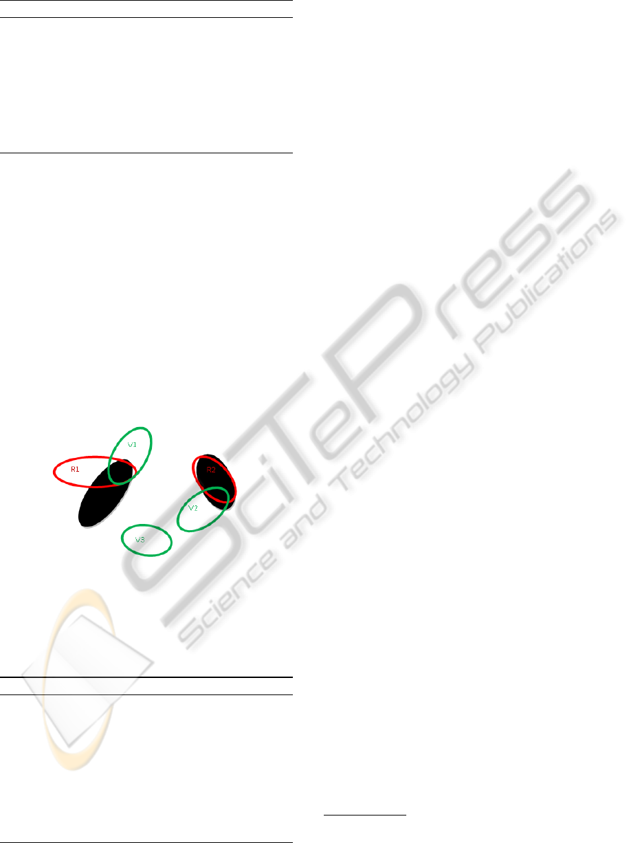
3.1 Birth Step
A new configuration x
0
of non-overlapping objects
is generated. Note that only objects which are
in the same configuration have to respect the non-
overlapping constraint, but two objects in different
configurations can intersect as can be seen on Figure
5.
Figure 5: Two configuration on an image (the black ellipses
are the object to detect).
The birth step is detailed in Algorithm 2. The
fourth step of this algorithm can be efficiently imple-
mented using a lookup table and the fast intersection
algorithm proposed in the latter.
Algorithm 2: Birth step.
Require: N, n
max
.
1: Set k = 0, n = 0, x
0
=
/
0.
2: while k < N and n < n
max
do
3: Construct an object ω
0
by generating a random
vector uniformly in χ.
4: If ω
0
intersects an object in x
0
, set n = n + 1 and
go back to 3.
5: Otherwise set x
0
= x
0
∪{ω
0
}, k = k +1, n = 0 and
go back to 3.
6: end while
3.2 Cut Step
This step consists in selecting the best configuration
of non-overlapping objects in (x
[n]
∪x
0
). To perform
this optimization, a weighted graph is constructed.
The nodes of this graph are the objects ω of the two
configurations x
[n]
and x
0
. This graph also possesses
two special nodes, the source ’s’ and the sink ’t’. The
weights should belong to [0,1] ∪{+∞} and are de-
fined using the data term U
d
(ω,u) by:
W (ω) = (1 −U
d
(ω,u))/2.
Graph Construction
Each object of the configuration (x
[n]
∪x
0
) is linked
to the source and the sink. The difference between
the objects ω
i
∈x
[n]
and the objects ω
j
∈x
0
is that the
objects ω
i
∈x
[n]
are linked to the source with a weight
equal to the data energy W (ω) and to the sink with a
weight equal to 1 −W (ω), while it is the reverse for
the objects ω
j
∈ x
0
.
The weights associated to edges linking two ob-
jects are non zero only when two objects intersect.
If ω
1
∈ x
[n]
(current configuration) intersects with
ω
2
∈ x
0
(new configuration), the link from ω
1
to ω
2
is set to ∞ and the link from ω
2
to ω
1
is set to zero
1
.
This ensures that the cut step generates an admissible
configuration (with no overlapping objects). Figure 6
summarises the graph construction of the configura-
tions on Figure 5. The nuclei to detect are represented
by black ellipses.
Cut
Once the graph is constructed, we perform a cut that
consists in partitioning the vertices into two disjoint
subsets. One contains the source and the other the
sink. The cut realized is the one with minimal cost
(the one minimizing the sum of the weights of the re-
moved edges).
After the cut step, if ω
i
∈ x
[n]
is in the sub-graph
containing the source, we keep it, otherwise we re-
move it. On the contrary the objects ω
j
∈ x
0
are
kept only if they belong to the sub-graph that con-
tains the sink. This difference of interpretation be-
tween the two configurations combined with the dif-
ferent weights to the source and the sink, ensure that
in case where an object of x
[n]
and an object of x
0
in-
tersect, only one can be kept.
The cut step is implemented using the graph-cut
1
When two objects intersect the link affected by a
weight of ∞ is always the link from the object of the cur-
rent configuration to the object of the new configuration.
ICPRAM2013-InternationalConferenceonPatternRecognitionApplicationsandMethods
100

Figure 6: Graph corresponding to the figure 5.
code developed by Yuri Boykov and Vladimir Kol-
mogorov in (Boykov et al., 2001; Boykov and Kol-
mogorov, 2004; Kolmogorov and Zabih, 2004).
3.3 A Fast Determination of Ellipses
Intersection
One of the proposed algorithm bottleneck is the fast
determination of whether two ellipsoids intersect or
not. In this section, we present a fast algorithm to
answer that question and prove theoretically that only
a few arithmetic operations suffice to provide the
answer with a low error rate.
Let ω be an ellipse or an ellipsoid. It can be
defined using a quadratic function Q
ω
as ω = {x ∈
R
d
,Q
ω
(x) = 1}. The quadratic function Q can be de-
fined by:
Q
ω
(x) = hA(x −c),(x −c)i (5)
where c denotes the object center and A is positive
definite matrix defined by:
A = P
−1
DP = P
T
DP.
where P is a rotation matrix and D is a positive diag-
onal matrix. In 2D, P is defined by:
P =
cos(θ) sin(θ)
−sin(θ) cos(θ)
and
D =
1
a
2
0
0
1
b
2
.
In 3D, the notation become cumbersome and we leave
them to the reader.
Let ω
1
and ω
2
be two ellipses or ellipsoids. In
order to know whether they intersect or not, we can
find the minimal level set of Q
ω
2
which intersects the
boundary of ω
1
. If this level set is associated to a
value greater than 1, the ellipses are separated, other-
wise they overlap. This idea can be formulated as the
following minimization problem:
min
x∈R
d
,Q
ω
1
(x)≤1
Q
ω
2
(x) (6)
This problem consists of minimizing a quadratic func-
tion over convex set. Projected descent methods can
thus be used. Unfortunately, there exists no closed
form solution to the problem of projection of a point
on an ellipse. We thus need to simplify the constraint
set:
min
Q
ω
1
(x)≤1
Q
ω
2
(x)
= min
hA
1
(x−c
1
),(x−c
1
)i≤1
hA
2
(x −c
2
),(x −c
2
)i
= min
h
√
A
1
(x−c
1
),
√
A
1
(x−c
1
)i≤1
hA
2
(x −c
2
),(x −c
2
)i
min
ky−
√
A
1
c
1
k
2
2
≤1
hA
2
(A
−
1
2
1
y −c
2
),(A
−
1
2
1
y −c
2
)i.
where y =
√
A
1
x. In this reformulation, the constraint
set Y = {y ∈R
d
,ky−
√
A
1
c
1
k
2
2
≤1}is a simple l
2
-ball
and the function F(y) = hA
2
(A
−
1
2
1
y − c
2
),(A
−
1
2
1
y −
c
2
)i is a strongly convex differentiable function. We
can thus use a projected gradient descent that writes:
Algorithm 3: Detection of overlapping ellipsoids.
Require: Q
ω
1
, Q
ω
2
, ε > 0.
1: Set k = 0, y
0
=
c
1
+c
2
2
.
2: Set µ =
b
2
1
a
2
2
, L =
a
2
1
b
2
2
.
3: Set τ =
2
µ+L
.
4: while ky
k+1
−y
k
k ≥ ε do
5: y
k+
1
2
= y
k
−τ∇F(y
k
).
6: y
k+1
= Π
Y
y
k+
1
2
.
7: k = k + 1.
8: end while
9: If F(y
k
) >= 1 return 0 (the ellipsoids do not inter-
sect with high probability).
10: If F(y
k
) < 1 return 1 (the ellipsoids intersect).
Let y
∗
denote the solution of the above prob-
lem. The previous algorithm comes with the follow-
ing guarantees:
Theorem 1. After k iterations, y
k
satisfies:
F(y
k
) −F(y
∗
) ≤
µ
2
ky
0
−y
∗
k
2
2
Q
F
−1
Q
F
+ 1
2k
ky
k
−y
∗
k
2
2
≤ ky
0
−y
∗
k
2
2
Q
F
−1
Q
F
+ 1
2k
where
Q
F
=
a
2
1
b
2
2
a
2
2
b
2
1
≤
λ
4
+
λ
4
−
.
A3DSegmentationAlgorithmforEllipsoidalShapes-ApplicationtoNucleiExtraction
101

Proof. The Hessian of F is H
F
(y) = 2A
−
1
2
1
A
2
A
−
1
2
1
.
Since A
1
and A
2
are products of orthogonal and diag-
onal matrices (A = P
T
DP), the eigenvalues of H
F
(y)
can be easily bounded:
λ
min
[H
F
(y)] ≥
b
2
1
a
2
2
λ
max
[H
F
(y)] ≤
a
2
1
b
2
2
The function F is thus µ-strongly convex with µ ≥
b
2
1
a
2
2
and its gradient is L-Lipschitz with L ≤
a
2
1
b
2
2
. Us-
ing standard convergence theorems in convex analysis
(Bertsekas, 1999), we obtain the announced result.
The conditioning number Q
F
depends solely on
the ratio between the major axis and the minor axis
sizes and not on the dimension d. This algorithm will
thus be as efficient in 3D as in 2D. For two circles
the ratio Q
F
is equal to
a
b
= 1 and the algorithm pro-
vides the exact answer after one iteration. For elliptic
ratios of 2, Q
f
= 16 and in the worst case, after 18
iterations, the algorithm returns a point y
k
that is 100
times closer to the intersection than y
0
. We also tested
an accelerated algorithm by (Nesterov, 2004), where
the convergence rate is of order
√
Q
F
−1
√
Q
F
+1
2k
but it did
not improve the computing times.
In our problems the ratio between a and b is al-
ways less than 2 and the algorithm usually converges
in just a few iterations (2 to 10 depending on the prob-
lem).
3.4 Acceleration by Local Perturbations
When the objects variability is important, the state
space size increases and affects the convergence speed
of the MBC algorithm. This problem is particulary
important in 3D since ellipsoids are defined by 9 pa-
rameters instead of 5 for the 2 dimensional case.
In order to improve the convergence speed,
(Gamal-Eldin et al., 2011) proposed to insert a selec-
tion phase in the birth step. This selection phase con-
sists in generating a dense configuration of objects at
similar locations and to keep the best ones using Be-
lief Propagation in order to form the new configura-
tion.
In this paper, we propose another heuristic in or-
der to increase the convergence speed. We propose to
alternate between two different kinds of birth steps.
The first one is that proposed in algorithm 2. The sec-
ond one consists in perturbating locally the current
configuration. This principle mimics the proposition
kernels used in RJMCMC algorithms (Perrin et al.,
2005). The idea behind this modification is that after
a while, most objects are close to their real location
and that local perturbations may allow much faster
convergence than fully randomized generation. This
algorithm is described in details in Algorithm 4.
Algorithm 4: MBC algorithm with local perturbations.
Require: N
1: Generate a configuration x
[0]
using Algorithm 2.
2: n ←− 0
3: while (Not converged) do
4: Generate a uniformly distributed random number
r ∈ [0, 1].
5: if r < p then
6: Generate a new configuration x
0
using Algorithm 2.
7: else
8: Generate a new configuration x
0
using Algorithm 5.
9: end if
10: x
[n+1]
←−Cut(x
n
∪x
0
)
11: n ←− n + 1
12: end while
Algorithm 5: Birth step with local perturbation.
Require: x
[n]
.
1: while k < size(x
[n]
) do
2: Construct an object ω
0
by local perturbation of
ω
k
∈ x[n].
3: If ω
0
intersects an object in x
0
, set k = k + 1 and
go back to 2.
4: Otherwise set x
0
= x
0
∪{ω
0
}, k = k + 1 and go
back to 2.
5: end while
Local Perturbations
A given object ω in x
[n]
is described by a set of pa-
rameters λ ∈ χ (see equations 1 and 2). We generate
the new object ω
0
by setting its parameters λ
0
= λ + z
where z is the realization of a random vector Z dis-
tributed uniformly in χ
ε
where :
χ
ε
= [−δ
xy
,δ
xy
]
2
×[−δ
ab
,δ
ab
]
2
×[0, 2π[
in 2D and
χ
ε
= [−δ
xyz
,δ
xyz
]
3
×[−δ
abc
,δ
abc
]
3
×[0, 2π[
3
in 3D.
The value of the different δ describes the perturba-
tion extent. We observed that small values accelerates
the convergence speed.
Comparison of the Convergence Speed
We have tested this method in order to compare the
speed of convergence of the MBC algorithm and the
MBC algorithm with local perturbation. Figure 7
ICPRAM2013-InternationalConferenceonPatternRecognitionApplicationsandMethods
102
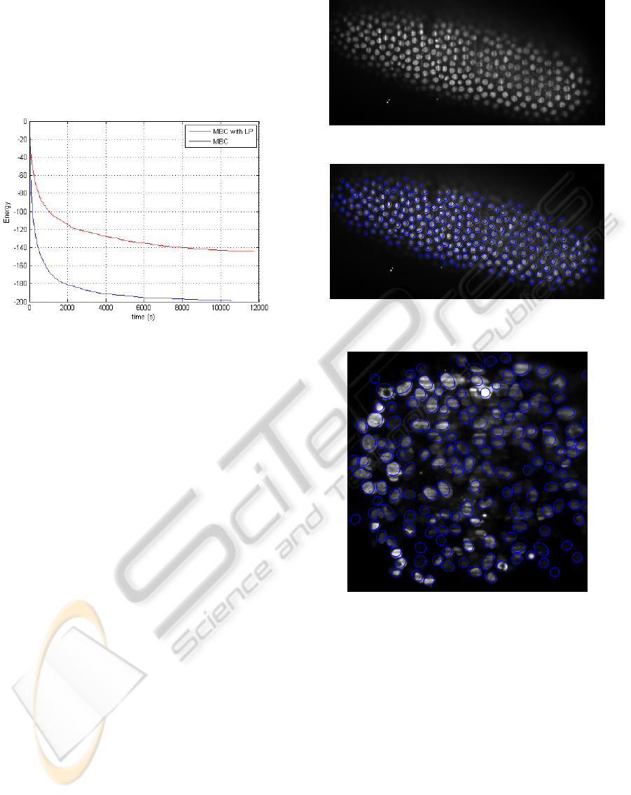
presents the energy evolution with respect to time for
both MBC and MBC with local perturbations (de-
noted MBC with LP) on the same image (the 3D nu-
clei of Drosophila embryo). The segmentation result
is presented on Figure 14 (image size 700 × 350 ×
100). These results show that the MBC with LP algo-
rithm strongly improve the MBC algorithm.
Figure 7: Comparison of the MBC and MBC with LP al-
gorithms.
4 RESULTS
In this section, we present some practical results in
2D and 3D. Figure 9 shows the segmentation result on
a Drosophila embryo obtained using SPIM imaging.
This is a rather easy case, since nuclei shapes vary
little. The images are impaired by various defects:
blur, stripes and attenuation. Despite this relatively
poor image quality, the segmentation results are al-
most perfect. The computing time is 5 minutes using
a c++ implementation. The image size is 700 ×350.
Figure 10 presents a more difficult case, where the
image is highly deteriorated. Nuclei cannot be iden-
tified in the image center. Moreover, nuclei variabil-
ity is important meaning that the state space size χ is
large. Some nuclei are in mitosis (see e.g. top-left).
In spite of these difficulties, the MBC algorithm pro-
vides acceptable results. They would allow to make
statistics on the cell location and orientation, which is
a major problem in biology. The computing times for
this example is 30 minutes.
Nuclei segmentation is a major open problem with
a large number of other applications. In Figure 11,
we attempt to detect the spermatozoon heads. The
foreseen application is tracking in order to understand
their collective motion. Figure 12 presents a multicel-
lular spheroid, an in vitro model mimicking micro-
tumor region organization, surrounded by a circle of
high aspect ratio pillars made in a soft material by ad-
vanced microfabrication processes. The aim of this
Figure 8: 2D nuclei of Drosophila embryo.
Figure 9: 2D segmentation of a nuclei of Drosophila em-
bryo (Fig 8).
Figure 10: 2D segmentation of a multicellular tumor
spheroid (Fig 1).
experiment is to determine the displacement of the
pillars induced by the spheroid dynamics. To address
this question, the precise detection of the contours of
the top of the pillars is required for this quantitative
measurement.
3D results are presented in Figure 14 and 16. For
the Drosophila embryo, the segmentation is very close
to what a human expert would do. The computing
times are 2 hours and the image size is 700 ×350 ×
100. The curves in Figure 14 correspond to this im-
age.
The spheroid segmentation presented in Figure 16
is less precise than the previous ones due to an im-
portant cell variability and to the fact that the images
A3DSegmentationAlgorithmforEllipsoidalShapes-ApplicationtoNucleiExtraction
103
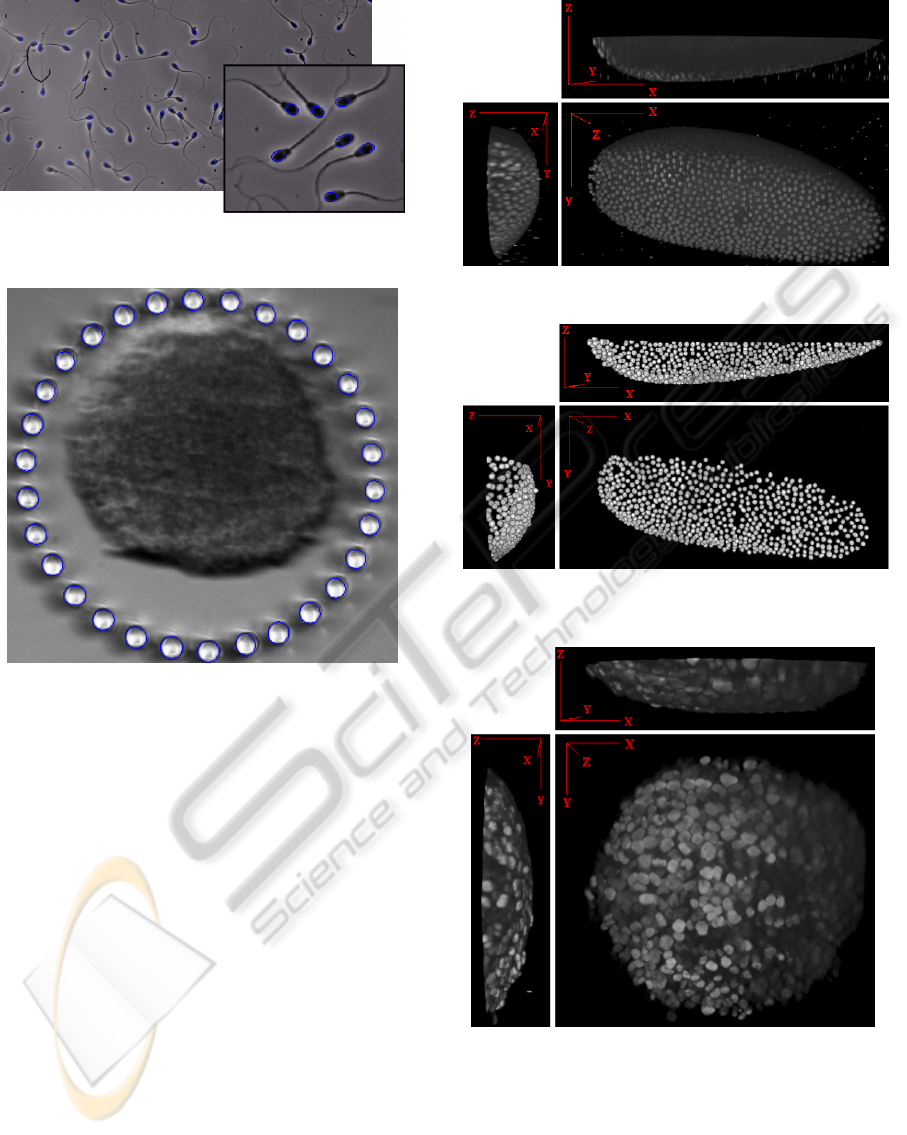
Figure 11: Segmentation of a spermatozoon colony (5 min-
utes). Image size: 2000 x 1024.
Figure 12: Micro pillars detection (less than 1 minute).
Image size: 840 x 800.
are extremly blurry in the Z direction. For that case,
image restoration algorithms and the design of new
energies robust to strong perturbations seem impor-
tant.
5 CONCLUSIONS
We proposed a detection algorithm capable of iden-
tifying sets of non intersecting ellipses or ellipsoids.
Interestingly, this algorithm contains only parameters
that are related to physical properties of the underly-
ing objects (e.g. nuclei variability in size and elliptic-
ity) and is thus easy to apply for any person working
in fields such as biological imaging. We presented the
wide applicability of this algorithm for 2D and 3D im-
ages. Even in hard cases with contrast loss and high
noise, the algorithm manages to find most nuclei due
to contrast invariant energies.
Future work will include a quantitative evaluation
of the algorithm efficiency with gold standards. We
are also investigating the possibility to encode more
Figure 13: 3D Drosophila embryo nuclei.
Figure 14: 3D segmentation of the Drosophila embryo nu-
clei (Fig 13).
Figure 15: 3D multicellular tumor spheroid.
complex interactions between objects to handle cases
where the normal to the image level lines do not pro-
vide sufficient information for ellipsoid fitting.
ICPRAM2013-InternationalConferenceonPatternRecognitionApplicationsandMethods
104
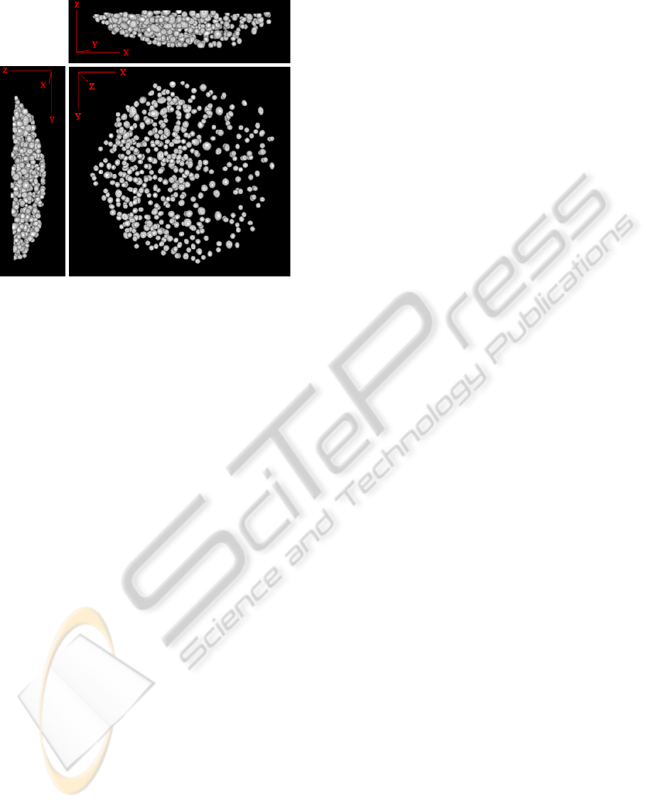
Figure 16: 3D segmentation of the multicellular tumor
spheroid (Fig 15).
ACKNOWLEDGEMENTS
This work was partially funded by the Mission
pour l’interdisciplinarit
´
e from CNRS, R
´
egion Midi
Pyr
´
en
´
ees, PEPII CASPA3D and ANR SPHIM3D.
The authors wish to thank F. Malgouyres and J.
Fehrenbach for interesting discussions. They also
thank V. Lobjois, C. Emery, J. Thomazeau, P. Escande
and B. Ducommun for their help in this project. They
thank L. Aoun and C. Vieu for providing images and
interesting discussions regarding micro pillars detec-
tion. They thank all the ITAV staff for their warm
welcome in a biology laboratory.
REFERENCES
Baddeley, A. and Van Lieshout, M. (1993). Stochastic ge-
ometry models in high-level vision. Journal of Ap-
plied Statistics, 20(5-6):231–256.
Bertsekas, D. (1999). Nonlinear programming.
Boykov, Y. and Kolmogorov, V. (2004). An experimental
comparison of min-cut/max-flow algorithms for en-
ergy minimization in vision. IEEE Trans. Pattern
Anal. Mach. Intell., 26(9):1124–1137.
Boykov, Y., Veksler, O., and Zabih, R. (2001). Fast ap-
proximate energy minimization via graph cuts. IEEE
Transactions on Pattern Analysis and Machine Intel-
ligence, 23:1222–1239.
Descombes, X. (2011). Stochastic geometry for image anal-
ysis. Wiley/Iste, x. descombes edition.
Descombes, X., Minlos, R., and Zhizhina, E. (2009). Object
extraction using a stochastic birth-and-death dynamics
in continuum. Journal of Mathematical Imaging and
Vision, 33(3):347–359.
Dong, G. and Acton, S. (2007). Detection of rolling leuko-
cytes by marked point processes. Journal of Elec-
tronic Imaging, 16:033013.
Gamal-Eldin, A., Descombes, X., Charpiat, G., and Zeru-
bia, J. (2011). A fast multiple birth and cut algorithm
using belief propagation. In Image Processing (ICIP),
2011 18th IEEE International Conference on, pages
2813–2816. IEEE.
Gamal Eldin, A., Descombes, X., Charpiat, G., Zerubia, J.,
et al. (2012). Multiple birth and cut algorithm for mul-
tiple object detection. Journal of Multimedia Process-
ing and Technologies.
Green, P. J. (1995). Reversible jump markov chain monte
carlo computation and bayesian model determination.
Biometrika, 82:711–732.
Kolmogorov, V. and Zabih, R. (2004). What energy func-
tions can be minimized via graph cuts. IEEE Trans-
actions on Pattern Analysis and Machine Intelligence,
26:65–81.
Nesterov, Y. (2004). Introductory lectures on convex opti-
mization: A basic course, volume 87. Springer.
Perrin, G., Descombes, X., and Zerubia, J. (2005). A
marked point process model for tree crown extraction
in plantations. In Image Processing, 2005. ICIP 2005.
IEEE International Conference on, volume 1, pages
I–661. IEEE.
A3DSegmentationAlgorithmforEllipsoidalShapes-ApplicationtoNucleiExtraction
105
