Spatially Varying Blur Recovery

Diagonal Approximations in the Wavelet Domain

Paul Escande

, Pierre Weiss

and Franc¸ois Malgouyres

ITAV-UMS3039, Universit

e de Toulouse, CNRS, Toulouse, France

IMT-UMR5219, Universit

e de Toulouse, CNRS, Toulouse, France

Keywords:

Image Deblurring, Spatially Varying Blur, Operator Approximation, Wavelet Packet Transform, Bi-harmonic

Spline Interpolation, Convex Optimization.

Abstract:

Restoration of images degraded by spatially varying blurs is an issue of increasing importance. Many new

optical systems allow to know the system point spread function at some random locations, by using micro-

scopic luminescent structures. Given a set of impulse responses, we propose a fast and efﬁcient algorithm to

reconstruct the blurring operator in the whole image domain. Our method consists in ﬁnding an approximation

of the integral operator by operators diagonal in the wavelet domain. Interestingly, this method complexity

scales linearly with the image size. It is thus applicable to large 3D problems. We show that this approach

might outperform previously proposed strategies such as linear interpolations (Nagy and O’Leary, 1998) or

separable approximations (Zhang et al., 2007). We provide various theoretical and numerical results in order

to justify the proposed methods.

1 INTRODUCTION

Image restoration in the presence of spatially varying

blur is a problem of increasing importance. It was ﬁrst

studied in the context of satellite imaging with Hubble

space telescope (Nagy and O’Leary, 1998). It is now

becoming increasingly important with the emergence

of new ﬂuorescence microscopes, producing highly

deteriorated images, since light interacts with the bi-

ological tissues. In microscopy, it is often possible

to incorporate micro-beads in the medium surround-

ing the sample or even in the sample itself, giving ac-

cess to the point spread function (PSF) of the system

at some known locations (see e.g. (Preibisch et al.,

2010; Temerinac-Ott et al., 2011)). This information

allows to interpolate the PSF in the whole space and

thus to get approximations of the degradation opera-

tor for further processing.

In the case of spatially invariant blur, fast decon-

volution algorithms can be devised since the convo-

lution is diagonal in the Fourier domain. This allows

using O(dn

log(n)) algorithms (where d denotes the

space dimension and n

denotes the number of pix-

els) based on the fast Fourier transform. These ap-

proaches are unsuitable in the case of spatially vary-

ing blurs and it appeals for the development of new

fast numerical algorithms. Our aim in this paper is to

propose fast O(n

) algorithms based on the wavelet

or wavelet packet transforms.

We consider a blurring operator H in R

and de-

ﬁned for any u ∈ L

(Ω) as the following integral op-

erator:

∀x ∈ Ω, (Hu)(x) :=

y∈Ω

K(x, y)u(y)dy, (1)

where Ω ⊆ R

is the image domain. The function

K(x, ·) is a spatially varying kernel deﬁning the PSF

at each location x. In all the following, we assume that

H is a bounded linear operator from L

(Ω) to L

(Ω).

The most naive approach to compute Hu numerically

consists in discretizing (1) by:

∀x ∈ X, Hu(x) =

∑

y∈X

K(x, y)u(y),

where X ⊂Ω denotes the set of pixels locations. This

approach is simple to implement, but costs O(n

)

arithmetic operations. This is unsuitable for large 2D

images or medium sized 3D images. Two alternative

approaches are commonly used:

• The ﬁrst one consists in approximating K(x, ·) by

a tensor product of kind:

K(x, (y

, ··· , y

)) =

∏

k=1

(x, y

222

Escande P., Weiss P. and Malgouyres F. (2013).

Spatially Varying Blur Recovery - Diagonal Approximations in the Wavelet Domain.

In Proceedings of the 2nd International Conference on Pattern Recognition Applications and Methods, pages 222-228

DOI: 10.5220/0004308202220228

 SciTePress

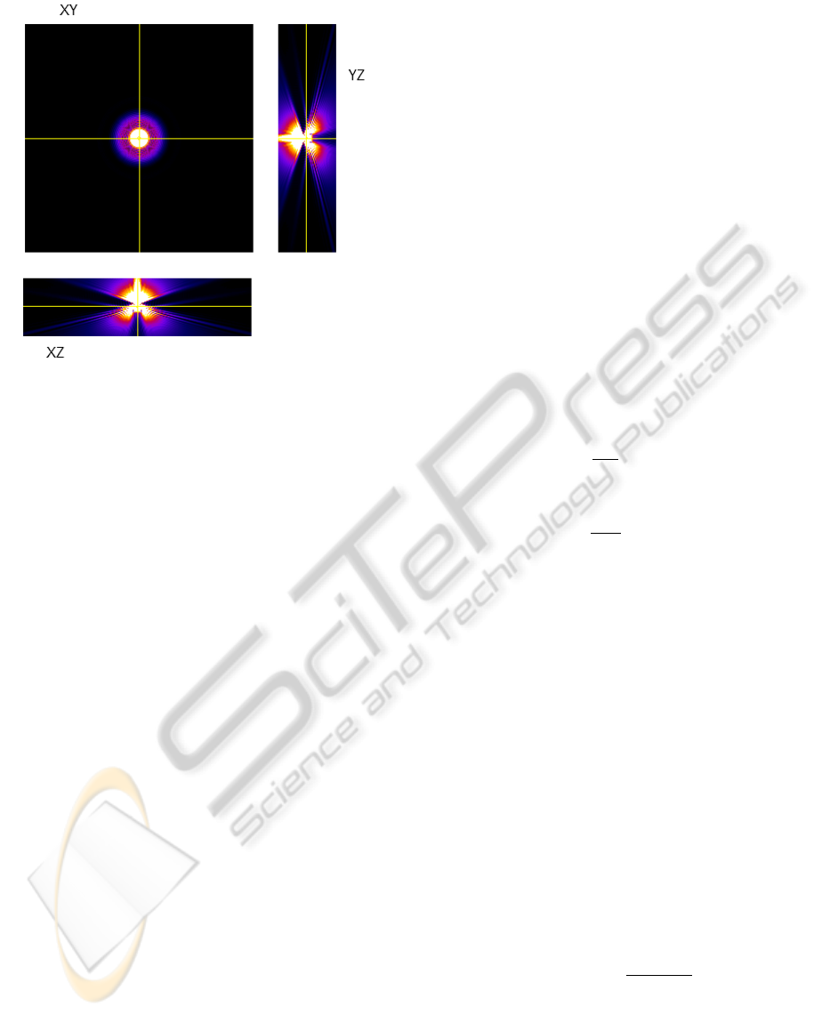
Figure 1: An orthogonal view of a Variable Refractive Gib-

son and Lanni PSF obtained with the PSF Generator plugin

for ImageJ (Kirshner et al., 2011).

This reduces the computational cost to O(dn

d+1

)

operations which is usually tractable even in large

scale scenarii. Moreover this model is exact for

Gaussian PSF which sometimes accurately de-

scribe perfect microscopy systems (Zhang et al.,

2007). Unfortunately, it is too rough to describe

more complex patterns commonly encountered

in optical diffraction or sample induced degrada-

tions. Figure 1 shows a typical PSF in three di-

mensions, which cannot be approximated by sep-

arable functions.

• The second one consists in using piecewise con-

stant blurs using local FFT (Nagy and O’Leary,

1998; Hansen et al., 2006). Its complexity is

roughly the same as that of spatially invariant

blurs in O(dn

log(n)). Moreover, this approach

also allows to use linear interpolations of the PSF.

This might be interesting in our case since the PSF

is known only at a few positions and linear in-

terpolations allow an operator reconstruction on

the whole image domain. Unfortunately, piece-

wise constant blurs or linear interpolations are too

rough to describe some practical settings. This is

illustrated on Figure 8(b), where we can observe

that the linear interpolation gives a cross like PSF

in the middle, that would be undesirable in practi-

cal cases.

In this work, we propose to approximate H by op-

erators diagonal in wavelet or wavelet packet trans-

forms. More precisely, we show that H ' ΨΣΨ

∗

where Ψ denotes the wavelet transform and Σ is a di-

agonal matrix. The computation of Hu is thus reduced

to O(n

) operations.

The structure of the paper is as follows. In section

3, we justify the use of such a structure by theoretical

and numerical results. In section 4, we propose an

algorithm to reconstruct the diagonal operator Σ when

the impulse response of H is given at some known

locations.

2 NOTATION

In order to simplify the notation, we consider wavelet

transforms and not wavelet packet transforms. We

present the theoretical results in 1D for the sake of

simplicity and clarity and the experimental results in

2D. The proposed approaches can be extended to any

dimensions and would be particularly suited to large

3D problems.

We consider an orthogonal wavelet basis of

(R ):

{φ

}

n∈Z

∪{ψ

j,n

}

j≤l

,n∈Z

where

j,n

(t) =

√

−j

ψ(2

−j

t −n), (2)

and ψ is the mother wavelet. The function φ

deﬁned by

(t) =

√

−l

φ(2

−l

t −n),

where φ is the scaling function.

In all the paper, Ψ

∗

denotes the forward wavelet

transform and Ψ denotes its inverse (in the discrete

and in the continuous setting). F

∗

denotes the Fourier

transform (discrete or continuous) and F denotes its

inverse. The convolution between u and h is denoted

h ? u. The Fourier transform of u is denoted ˆu or F

∗

For a discrete image in R

, we deﬁne the discrete

partial derivative in direction i by:

∂

u(·, k, ·) =



u(·, k + 1, ·) −u(·, k, ·) if 1 ≤k < n

0 if k = n.

where the indice k is that the i-th position in the array.

The discrete gradient operator in R

is deﬁned by:

∇ = (∂

;∂

;··· ; ∂

)

Let q ∈ (R

)

represent a discrete vector ﬁeld. We

set

q = (q

;··· ; q

The isotropic l

-norm in (R

)

is deﬁned by:

kqk

1,2

∑

i=1

∑

j=1

(i)

Finally, the discrete total variation of u ∈ R

is de-

ﬁned by:

TV (u) = k∇uk

1,2

SpatiallyVaryingBlurRecovery-DiagonalApproximationsintheWaveletDomain

223

3 DIAGONALIZATION OF THE

VARIABLE BLUR OPERATOR

IN A WAVELET BASIS

The main ingredient allowing the design of efﬁcient

deconvolution algorithms is the fact that a convolu-

tion is diagonalized in the Fourier domain. For any

kernel h, h ? u = F ΣF

∗

u where Σ can be considered

as a diagonal operator that multiplies F

∗

u by F

∗

The main idea of this paper is to mimic this property

for spatially varying blur operators. We propose to ap-

proximate H by an operator

H diagonal in the wavelet

domain:

Hu '

:= ΨΣΨ

∗

∑

n∈Z

hφ

, uiφ

∑

j≤l

,n∈Z

j,n

hψ

j,n

, uiψ

j,n

where (σ

j,n

)

j,n

is a sequence of weights that will be

described later. This particular structure allows to ap-

proximate Hu in O(n

) arithmetic operations, which

is doable even for very large scale problems.

Such operators have been deeply analyzed from a

theoretical point of view in various articles or mono-

graphs (see e.g. (Beylkin et al., 1991; Coifman and

Meyer, 1997)). However, we found very few im-

age processing applications in the literature. To our

knowledge, the closest practical application is ded-

icated to the fast computation of image foveation

(Chang et al., 1999). However, this work is only

adapted to very particular kind of kernels K met in

foveation that do not correspond to our practical prob-

lems.

Since H is a linear operator in a Hilbert space, it

can be written as:

H = ΨΘΨ

∗

where Θ : l

→ l

is characterized by the coefﬁcients,

(θ

j,m,k,n

)

j,m,k,n

:= (hHψ

j,m

, ψ

k,n

j,m,k,n

In order to justify the proposed approach, we ﬁrst

recall some theoretical results presented in (Beylkin

et al., 1991) that assess the decrease of θ

j,m,k,n

away

from the diagonal (i.e. when |m −n|> 0 and |j −k|>

0). Then we provide an interpretation of the coefﬁ-

cients σ

j,n

in terms of amplitudes of the Fourier coef-

ﬁcients of the local PSF.

3.1 Decay of Θ Away from the Diagonal

In (Beylkin et al., 1991), it has been proved that, for

compactly supported wavelets possessing M vanish-

ing moments and smoothly varying kernels, the val-

ues of Θ are small away from the diagonal in the one

and two-dimensional cases. Typical results are as fol-

low:

Theorem 1 ((Beylkin et al., 1991)). Suppose that

|K(x, y)|≤

|x−y|

and that K(x, y) is of class C

M+1

with

|∂

K(x, y) + ∂

K(x, y)| ≤

|x −y|

(1+M)

where M denotes the number of vanishing moments of

ψ. Then θ

j,m,k,n

satisﬁes the following inequality:

|θ

j,m,k,n

| ≤ O



1 + |j −k|

M+1



Moreover, for compactly supported kernels K:

|θ

j,m,k,n

| = 0,

for sufﬁciently large |m −n|.

The authors also show that the operator norm

kH −Ψ

ΘΨ

∗

k can be made arbitrarily small if

Θ is

obtained by thresholding Θ in such a way that only

O(n

) coefﬁcients are kept. It roughly means that if K

is a smooth kernel, computing Hu can be performed

in O(n

) operations, rather than O(n

), by making

use of the wavelet transform. In this work, rather than

considering sparse matrices

Θ, we use simpler diago-

nal matrices.

We illustrate these results experimentally in the

discrete setting on Figure 3. We consider an operator

H whose kernel is a two-dimensional Gaussian with

variances linearly increasing in the vertical direction,

see Figure 2(c). This operator applied to the mandrill

image results in the image Figure 2(b). The matrix Θ

is shown on Figure 3. It is seen that Θ is dominated

by its diagonal entries and that the coefﬁcients away

from the diagonal decrease extremely fast (actually

much faster than the result in Theorem 1).

3.2 Interpretation of the Diagonal

Values

In this paragraph, we show that the values σ

j,n

can

be interpreted as local frequency responses of

H. We

assume that ψ is a compactly supported wavelet on

the interval [−β, β].

Let us analyze the impulse response of

H at point

Hδ

= ΨΣΨ

∗

∑

n∈Z

(x)φ

∑

j≤l

,n∈Z

j,n

(x)ψ

j,n

∑

n∈Z

(x)φ

∑

j≤l

n∈k(x, j)

j,n

(x)ψ

j,n

ICPRAM2013-InternationalConferenceonPatternRecognitionApplicationsandMethods

224

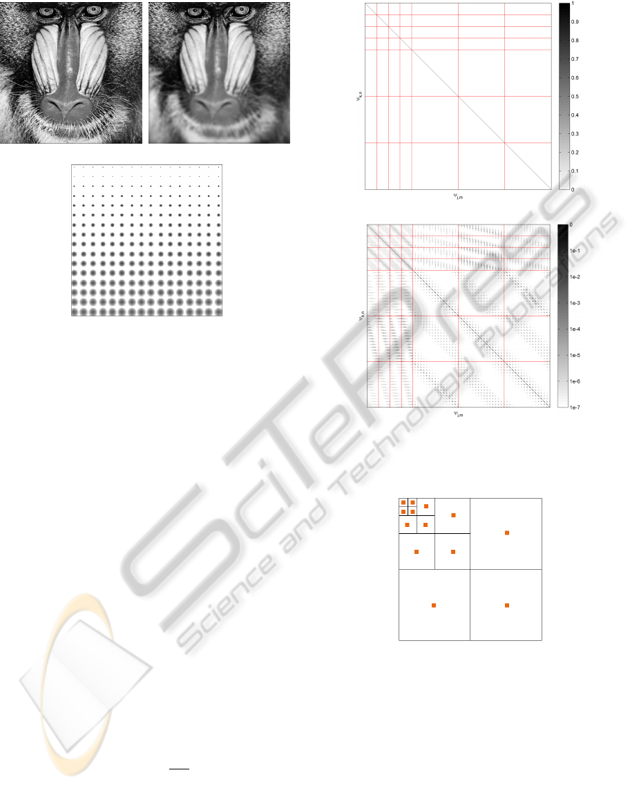
(a) Original Image (b) Blurred Image

Figure 2: Image blurred using the operator H. The kernel

K of the operator is a Gaussian which grows linearly in the

vertical direction.

where

k(x, j) :=



n ∈ Z such that



−j

x −n



< β



The sets k(x, j) are represented in Figure 4 in the two-

dimensional case. They contain at most b2βc ele-

ments.

Now, if we assume that σ

j,n

varies little in k(x, j)

and satisﬁes σ

j,n

' σ

j,x

we obtain:

ΨΣΨ

∑

n∈k(x,l

)

(x)φ

∑

j≤l

j,x

∑

n∈k(x, j)

j,n

(x)ψ

j,n

The local frequency response of

H is thus

ΨΣΨ

∗

∑

n∈Z

(x)

∑

j≤l

j,x

∑

n∈k(x, j)

j,n

(x)

j,n

∑

n∈Z

(x)

∑

j≤l

j,x

where α

j,x

is a complex coefﬁcient that depends on

the choice of ψ and ψ

(x) =

√

−j

ψ(2

−j

x). Since

is well localized in the frequency domain, the coefﬁ-

cient σ

j,x

can be interpreted as a local frequency

attenuation in a certain frequency band that depends

solely on the scale j. This principle is illustrated in

Figure 5.

(a) In a linear scale

(b) In a log

scale

Figure 3: Matrix Θ for the operator illustrated in Figure 2.

This matrix is obtained using Daubechies 8 wavelets and a

decomposition level J = 2.

Figure 4: The sets k(x, j) are indicated in orange at each

scale.

3.3 Spatial Regularity of the

Eigenvalues

A simple way to ﬁnd a matrix Σ such that

H ' H

consists in setting Σ = Diag(Θ). If the kernel K

varies sufﬁciently smoothly in space, the discrete val-

ues (σ

j,n

)

n∈Z

also vary smoothly, meaning that σ

j,n

j,n+1

. This can be veriﬁed experimentally: Fig-

ure 6 represents the diagonal of Θ for an operator

H displayed in Figure 2(c) in the usual wavelet do-

SpatiallyVaryingBlurRecovery-DiagonalApproximationsintheWaveletDomain

225

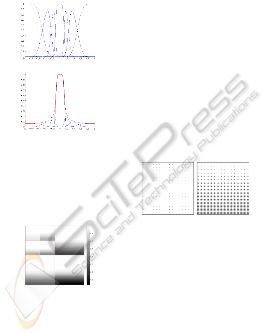
(a) In blue



and in red

∑



(b) In blue |σ

j,x



| and in red

∑

j,x

Figure 5: Local Fourier attenuation are determined by the

coefﬁcients σ

j,x

main. The eigenvalues vary smoothly in each sub-

band. This remark is central to understand the inter-

polation algorithm proposed in the next section.

Also notice that the coefﬁcients σ

j,n

decrease

from the top to the bottom of the image at each scale.

It means that the high-frequencies are attenuated on

the image bottom. This clearly corresponds to the op-

erator H shown in Figure 2(c).

Figure 6: Diagonal of the matrix Θ.

4 OPERATOR

RECONSTRUCTION FROM

LOCALLY KNOWN PSF

In this section, we propose a method to recover the

matrix Σ from the knowledge of local impulse re-

sponses. This setting corresponds to various practical

applications. In astronomy, stars may sometimes be

considered as Diracs. Their observation thus provides

the impulse response of the system K(x, ·), where x

denotes the star location. In microscopy, micro-beads

may be inserted in the sample and provide the impulse

responses at locations spread in the whole image do-

main.

The problem tackled in this section is the recon-

struction of K everywhere, from the knowledge of

K(x

, ·) at a few locations (x

)

i∈{1,···,m}

. We assume

that two images are available:

• An image

u =

∑

i=1

that describes the Dirac locations.

• An image u

= Hu which provides the impulse

responses at locations x

Figure 7 illustrates two images u and u

. The Diracs

could be randomly located on the image rather than on

a uniform grid. We considered this simple setting for

experimental reasons. The number of known impulse

responses can also be considerably reduced as will be

shown later.

(a) The dirac map u (b) u

= Hu

Figure 7: Dirac map and the associated impulse responses.

This information is used to reconstruct an approximation of

the blurring operator H.

The knowledge of u

allows to reconstruct the

eigenvalues σ

j,n

H only close to the known loca-

tions x

in each sub-band. These eigenvalues should

thus be interpolated in order to recover K everywhere.

Note that this problem is not standard since is consists

in interpolating an operator eigenvalues and not an

image.

Since the eigenvalues vary smoothly in space, we

propose to use bi-harmonic splines which are well

adapted to scattered data interpolation (Wahba, 1990).

The approximation problem we propose formulates as

the following variational problem:

Find Σ ∈argminkΨΣΨ

∗

u −u

+ λR(Σ), (3)

where λ > 0 is a regularization parameter. We also

set:

R(Σ) =

∑

j≤l

k∆σ

ICPRAM2013-InternationalConferenceonPatternRecognitionApplicationsandMethods

226

where ∆ denotes the discrete Laplacian and σ

de-

notes the set of eigenvalues at scale j. This energy

provides the approximation of minimal curvature. It

is equivalent to using bi-harmonic splines (Wahba,

1990).

The quadratic structure of problem (3) allows the

use of conjugate gradient like methods for the min-

imization. We are currently investigating the use of

preconditionners in the wavelet domain for accelerat-

ing the convergence.

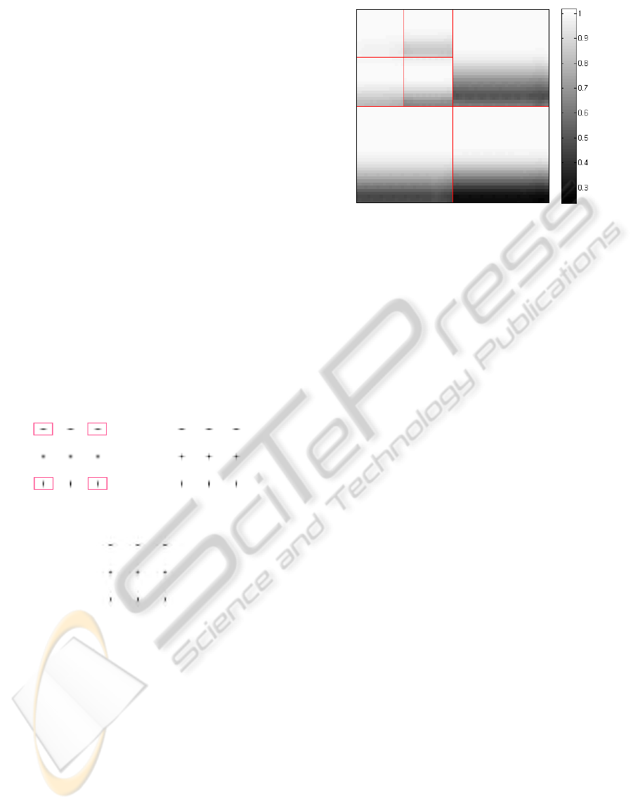
We present approximation results in Figures 8 and

9. Figure 9 displays a interpolated matrix Σ. This

result can be evaluated by comparing it with the true

diagonal of Θ presented in Figure 6. Overall, the re-

construction leads to near perfect results. Figure 8

compares the interpolation provided by Fourier based

methods such as (Nagy and O’Leary, 1998) with the

proposed approach. Our method produces some ar-

tifacts, however, the proposed interpolation is rather

close to the reality in the image center. Note that this

result is obtained using knowing the PSF at only 4 lo-

cations in the plane. Deblurring an image with kernel

8(b) would be disastrous, since horizontal and verti-

cal frequencies would be enhanced, leading to strong

ringing artifacts.

(a) Exact PSF (b) Linearly Interpolated

PSF

Figure 8: Operator reconstruction using different methods.

The operator is reconstructed using the information avail-

able in the red rectangles.

5 RESULTS

In this section, we assume that the diagonal Σ has

been reconstructed using the method proposed in sec-

tion 4. We propose a total variation (TV) based algo-

rithm to tackle the deblurring problem. We suppose

that a degraded image v

is obtained according to the

following model v

= Hv+η where H : R

→R

the spatially varying blur operator, v ∈ R

is the un-

altered image and η ∈ R

is a white Gaussian noise,

Figure 9: The matrix Σ reconstructed using bi-harmonic

splines. It should be compared to the real diagonal pre-

sented on Figure 6.

η ∼ N (0, σ

). Our aim is to recover v knowing

. Since

H and H are usually compact, the problem

of recovering v is ill-posed and should be regularized.

We propose to use a standard total variation based re-

construction approach. It reads:

Find argmin

v∈R

Hv−v

≤α

TV (v), (4)

where α > 0 is a user ﬁxed parameter and TV (v) is the

isotropic total variation of v deﬁned in the notation. In

settings where H is perfectly known, users should set

α = σ

n. The proposed approach differs since total

variation serves as a regularizer for both the noise and

the errors in the operator approximation. In practice

we found that setting α = (1 + ε)σ

n where ε > 0 is a

small parameter provides good experimental results.

Problem (4) is solved using the primal-dual algorithm

proposed in (Chambolle and Pock, 2011).

In order to assess the method, we used the Man-

drill and Lena images rescaled in [0, 1] and blurred

with an operator having a two-dimensional Gaussian

PSF. In Figures 11 and 12 we respectively added a

noise of variance σ

= 0 and σ

= 3.10

−2

. In the case

= 0, Figure 11 shows that the algorithm is able to

recover thin details of the image even in the coat and

the beard of the Mandrill. This highlights the fact that

the approximation of H by

H is sufﬁciently good for

the sake of deblurring. In the case of a larger noise,

= 3.10

−2

, Figure 12 shows that the image qual-

ity is improved but suffers from the standard defects

of total-variation based regularization: stair-case ap-

pears and thin details are not recovered. Images of

larger size can be found on the website of the authors.

ACKNOWLEDGEMENTS

This work was partially funded by the Mission pour

SpatiallyVaryingBlurRecovery-DiagonalApproximationsintheWaveletDomain

227

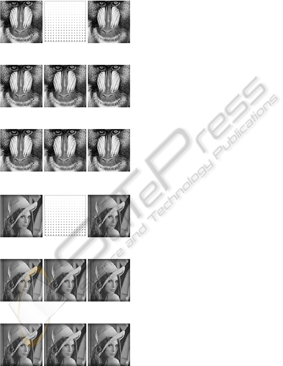
Figure 10: Original image, impulse responses and blurred

image.

Figure 11: Restoration results for σ

= 0. Degraded Image

SNR = 22.51dB, restored image SNR = 29.02dB.

Figure 12: Restoration results for σ

= 3.10

−2

. Degraded

Image SNR = 20.58dB, deblurred Image SNR = 20.86dB.

Figure 13: Original Image, impulse responses, blurred im-

age.

Figure 14: Restoration for σ

= 0. Original, degraded

SNR = 30.30dB, deblurred SNR = 36.13dB).

Figure 15: Restoration for σ

= 10

−2

. Original, degraded

SNR = 28.14, deblurred SNR = 29.18.

l’interdisciplinarit

e from CNRS, R

egion Midi

Pyr

ees and the ANR SPHIM3D.

The authors wish to thank J. Bigot and J. Fehren-

bach for interesting discussions. They also thank all

the ITAV staff, Charlotte Emery and Emmanuel Sou-

bies for their tireless support during this project.

REFERENCES

Beylkin, G., Coifman, R., and Rokhlin, V. (1991). Fast

wavelet transform and numerical algorithm. Commun.

Pure and Applied Math., 44:141–183.

Chambolle, A. and Pock, T. (2011). A ﬁrst-order primal-

dual algorithm for convex problems with applications

to imaging. Journal of Mathematical Imaging and Vi-

sion, 40(1):120–145.

Chang, E.-C., Mallat, S., and Yap, C. (1999). Wavelet

foveation. Applied and Computational Harmonic

Analysis, 9:312–335.

Coifman, R. and Meyer, Y. (1997). Wavelets, calder

on-

zygmund and multilinear operators. Cambridge Stud-

ies in Advanced Math, 48.

Hansen, P., Nagy, J., and O’leary, D. (2006). Deblurring

images: matrices, spectra, and ﬁltering. Siam.

Kirshner, H., Sage, D., and Unser, M. (2011). 3D PSF

models for ﬂuorescence microscopy in ImageJ. In

Proceedings of the Twelfth International Conference

on Methods and Applications of Fluorescence Spec-

troscopy, Imaging and Probes (MAF’11), page 154,

Strasbourg, France.

Nagy, J. and O’Leary, D. (1998). Restoring images de-

graded by spatially variant blur. SIAM Journal on Sci-

entiﬁc Computing, 19:1063.

Preibisch, S., Saalfeld, S., Schindelin, J., and Tomancak, P.

(2010). Software for bead-based registration of selec-

tive plane illumination microscopy data. Nature meth-

ods, 7(6):418–419.

Temerinac-Ott, M., Ronneberger, O., Ochs, P., Driever, W.,

Brox, T., and Burkhardt, H. (2011). Multiview de-

blurring for 3-d images from light sheet based ﬂuores-

cence microscopy. Image Processing, IEEE Transac-

tions on, (99):1–1.

Wahba, G. (1990). Spline models for observational data,

volume 59. Society for Industrial Mathematics.

Zhang, B., Zerubia, J., and Olivo-Marin, J. (2007).

Gaussian approximations of ﬂuorescence microscope

point-spread function models. Applied Optics,

46(10):1819–1829.

ICPRAM2013-InternationalConferenceonPatternRecognitionApplicationsandMethods

228