
RqPCRAnalysis: Analysis of Quantitative Real-time PCR Data
Frédérique Hilliou
1
and Trang Tran
2
1
UMR-IBSV-INRA-CNRS, Université de Nice Sophia Antipolis, Nice, France
2
INGENOMIX, Lanaud, 87220 Boisseuil, France
Keywords: Quantitative Real-time PCR, Normalization, Biological Replicates, Statistics, R.
Abstract: We propose the statistical RqPCRAnalysis tool for quantitative real-time PCR data analysis which includes
the use of several normalization genes, biological as well as technical replicates and provides statistically
validated results. This RqPCRAnalysis tool improved methods developed by Genorm and qBASE
programs. The algorithm was developed in R language and is freely available. The main contributions of
RqPCRAnalysis tool are: (1) determining the most stable reference genes (REF)--housekeeping genes--
across biological replicates and technical replicates; (2) computing the normalization factor based on REF;
(3) computing the normalized expression of the genes of interest (GOI), as well as rescaling the normalized
expression across biological replicates; (4) comparing the level expression between samples across
biological replicates via the test of statistical significance. In this paper we describe and demonstrate the
available statistical functions for practical analysis of quantitative real-time PCR data. Our statistical
RqPCRAnalysis tool is user-friendly and should help biologist with no prior formation in R programming to
analyze their quantitative PCR data.
1 INTRODUCTION
In molecular biology the real-time quantitative
polymerase chain reaction (RT-qPCR) has become
the most powerful method for the detection and
quantification of nucleic acid sequences including
gene expressions. The technique is widely used for
example for the validation of genes differentially
expressed in microarray experiments. Several
programs have been developed to extract
quantification cycle values (Cq) from recorded
fluorescence measurements and are specific for each
qPCR machine manufacturers. The process of these
raw data is however not always adequate for the
biologist because they lack for example
normalization steps and are often dedicated to a
single instrument. Recently Bustin et al. provided
standard for qPCR technique: MIQE (Minimum
Information for Publication of Quantitative Real-
Time PCR Experiments) (Bustin et al., 2010);
(Bustin et al., 2002). Design of qPCR data
experiment should include technical replicates,
biological replicates as well as several reference
genes used for data normalisation.
Base of the MIQE we propose an R application
that should allow users whatever instruments they
used to determine reference genes in their set of data
and to quantify expression levels of their genes of
interests. R is a widely used open source language
and environment for statistical computing and
graphical representation which has become a
standard in statistical modeling, data analysis,
biostatistics and machine learning. An important
feature of the R environment is that it integrates
generic data analysis and visualization
functionalities with the latest advances in
computational statistics.
This paper introduces the new R package
RqPCRAnalysis, where the acronym stands for
analysis of real-time quantitative PCR data. The
purpose of the package RqPCRAnalysis is to
provide a comprehensive, simple and easy to use
tool for real-time quantitative PCR data analysis.
More importantly, functions are provided for
biologists who have little statistical and R
programming background. Our R-script was
developed base on Genorm algorithm
(Vandesompele et al., 2002) to search for reference
genes and on qBASE algorithm for calculation of
gene relative expression levels (Hellemans et al.,
2007). We developed a statistical method for the
validation of differential expressions for genes of
202
Hilliou F. and tran T..
RqPCRAnalysis: Analysis of Quantitative Real-time PCR Data.
DOI: 10.5220/0004312002020211
In Proceedings of the International Conference on Bioinformatics Models, Methods and Algorithms (BIOINFORMATICS-2013), pages 202-211
ISBN: 978-989-8565-35-8
Copyright
c
2013 SCITEPRESS (Science and Technology Publications, Lda.)

interest (GOI) and we compared the expression level
between samples via the test of statistical
significance. A graphic representation of these
results is also available.
2 METHODS
2.1 Biological Data
2.1.1 Plant Growth Conditions
and Wounding Treatment
Arabidopsis thaliana wild-type (ecotype Columbia 0,
Col0) and CYP74A1-OverExpressed mutant (M)
seeds were cold-treated at 4°C for two days. After
cold treatment, seeds were sown on soil previously
autoclaved 1h at 130°C and then placed in a
controlled growth room under long-day conditions:
-12h of light with a minimum intensity of
100mmolm
-2
s
-1
at 21°C.
-12h of dark at 21°C.
Plants were watered once a week. Wounding
was done on 4-week-old plants (8 to 10 mature
leaves) as described in Park et al., 2002. Wounded
leaves were harvested 2h and 4h after wounding and
were immediately frozen in liquid nitrogen.
Undamaged leaves were also harvested as control.
This control is described at t=0h. Twenty plants of
each genotype were pooled for each time point.
Three biologically independent experiments were
done and used as biological replicates.
2.1.2 RNA Extraction
RNA was extracted using Trizol reagent (Invitrogen
Life technologies) according to manufacturers'
instructions. Three independent extractions were
performed on three independent biological replicates
for each time point of the time course and for each
genotype.
2.1.3 Real Time Quantitative PCR
For each RNA template we reverse-transcribed 2μg
of total RNA during 2h at 42°C using 200 units of
SuperScript
TM
II (Invitrogen), 5μM oligo(dT)
18
,
500μMdNTP's, 40 units of Ribonuclease inhibitor
(RNasin, Promega). Fifty nanograms of cDNA
synthesis were then used in qPCR experiments using
qPCR
TM
Mastermix Plus for SYBR Green I
(Eurogentec) and 3.6μM of each gene-specific
primers in a final volume of 15μl. qPCR reactions
were carried out on an Opticon monitor 2 (BioRad)
The PCR conditions were as follows: 95°C for 15
min to activate the hot-start DNA polymerase,
followed by 40 cycles of 95°C for 30s, 60°C for 30s
and 72°C for 30s. Each reaction was performed in
technical duplicates and the mean of three
independent biological replicates was calculated. For
each gene, primers efficiency was assessed and new
set of primers were designed until efficiency
between 85-105% was obtained. Czechowski (2004)
proposed several "stable" genes for Arabidopsis
obtained using plant growth in several conditions
(Czechowski et al., 2004). We chose three most
stable genes At5g46630, At1g58050, and
At1g62930 and their respective primers among these
to be used as reference genes in our experiment. The
stability of these three genes was also tested using
GeNorm (Vandesompele et al., 2002) and our R
package RqPCRAnalysis.
Table 1: Primer characteristics.
gene name
accession
number
primer s e que nce s
amplicon
size
PCR
efficiency
correlation
coefficient
TCGATTGCTTGGTTTGGAAGAT
GCACTTAGCGTGGACTCTGTTTGATC
CCATTCTACTTTTTGGCGGCT
TCA ATGGTAACTGATCCACTCTGATG
GA GT TGCGGGT TT GTT GGA G
CAAGACAGCATTTCCAGATAGCAT
GGAA GCTCCGTTA A TTTCTCG
GGACTA CACAGGTGCGAACA
GA T GGCGA A A GGA GA TGA GA
CCCTATGACATGAAGGGACTG
GA A GGA GCCA A A CA T GGA T C
AATA CA CACGA TTTAGCACC
HKG1
AT5G46630
HKG2
AT1G58050
60 96% 0,991
60 80% 0,99
105% 0,994
cyp74a
At5g42650
92 93% 0,996
HKG3
AT1G62930
98
0,984
pdf1.2a
At5g44420
108 87% 0,978
cyp76c5
At1g33730
105 83%
RqPCRAnalysis:AnalysisofQuantitativeReal-timePCRData
203

GOI primers were designed using Primer3
software (http://frodo.wi.mit.edu/cgi-bin/primer3/
primer3-www.cgi) and absence of secondary
structures was checked using Netprimer software
(http://www.premierbiosoft.com/netprimer/netprlaun
ch/\\netprlaunch.html). Primers characteristics are
summarized in Table 1 for REF genes and GOI.
2.2 Statistical Methods
Let us note m, n respectively the number of
biological replicates and number of technical
replicates; r, number of reference genes; E
j
is the
PCR amplification efficiency coefficient of gene j;
Cq, quantitative cycle; QCq, relative quantity; SD,
standard deviation; SE, standard error; NF,
normalization factor.
2.2.1 Identification of Reference Genes
The normalization of relative quantities with the
reference genes (REF), the most stable genes, can be
calculated on the assumption that the REFs are
known (i.e. provided by the biologist). When the
REFs are not know, we can determine the most
stably expressed genes across all tested samples and
all biological replicated experiments based on the
stability parameter and coefficient of variation.
Here, we use the algorithm described in (Hellemans
et al., 2007) to identify the reference genes.
2.2.2 Computation of Relative Quantities
For each biological replicate i, the average of Cq is
computed for n technical replicates of the same gene
j:
∑
1
1
(1)
The relative quantity associated with
is
expressed as follows where the highest expression
level set to one,
(2)
and the standard deviation of QCq
ij
is obtained by
taking the derivative of (2):
∗
∗ln
(3)
2.2.3 Computation of Normalization Factor
The normalization factor of sample k in biological
replicate i across r reference genes, noted NF
ik
, is
given by the geometric mean
(4)
And the standard deviation of this normalization
factor is
(5)
with r corresponding to the number of reference
genes.
2.2.4 Normalization of Relative Quantities
For each biological replicate i, the normalization of
relative quantity of GOI j for each sample k can be
now calculated by dividing the raw GOI quantity (2)
by the normalization factor (4) as follows
∗
(6)
and the standard deviation of this normalized GOI
expression is given by
∗
∗
(7)
Here, we are also interesting in the error on the mean
by using the standard error (SE) values instead of
standard deviation (the error on a single measured
value) as the following. Using this SE, the true mean
has a 95% chance of lying between the measured
mean ±1.96 times the SE.
∗
∗
√
(8)
Now, the average of expression level of GOI j for
each sample k across m biological replicates is
calculated by
∗
∑
∗
(9)
BIOINFORMATICS2013-InternationalConferenceonBioinformaticsModels,MethodsandAlgorithms
204

and the SD and SE are basically given by
∗
1
1
∗
∗
∗
∗
√
(10)
Finally, the user can use the reference sample k, the
logarithm transformation or the smallest sample for
rescaling the expression level
∗
.
∗
.
∗
,
∗
.
∗
.
min
∗
(11)
The SD and SE corresponding to the transformation
in (11) are
∗
.
.
∗
∗
∗
.
∗
.
√
∗
.
.
∗
min
∗
∗
.
∗
.
√
(12)
2.2.5 Sample Comparison
For each GOI, all pairs of samples across all
biological replicates are compared. Here we used the
classical method of pairwise t-test with pooled
standard deviation. We assumed that the two sample
sizes are equal and the two distributions have the
same variance. In order to apply the t-test, we
assume data follow normal distribution. Here we use
a simple logarithm transformation to transform the
normalized relative expression,
∗
log
∗
forall
(13)
Now, the t statistic to test whether the means are
different between the samples S_i and S_j follows a
Student's t-distribution with M-1 degrees of freedom
and can be calculated as follows:
̅
̅
/
√
(14)
where SD(S
i
-S
j
) is the standard deviation of the
differences between the S
i
and the S
j
:
Once a t value is determined, the p-value of the test
can be calculated from Student's t-distribution with
M-1 degrees of freedom. The user can choose a
threshold for the statistical significance to reject or
accept the null hypothesis (H
0
: μ
i
=μ
j
) in favor of the
alternative hypothesis (H
a
: μ
i
≠μ
j
).
3 RESULTS
3.1 Determination of Relative
Expression
An example of raw data is available in Table 3
(APPENDIX). This example consists of three
biological replicates and two technical replicates.
We compared expression levels of six genes (3 REF
genes and 3 GOIs namely CYP74A, CYP76C5, and
PDF1.2a) in Col versus the mutant M CYP74A1-
OE. We performed our qPCR analysis in six
different biological conditions. In this example, the
REF genes were obtained using GeNorm software
and were confirmed using our R-script. Figure 1
presents results of rescaled expression of GOI1,
GO2 and GOI3 where all six biological conditions
and their respective standard deviations are plotted.
We observed that the GOI1 (CYP74A) is over-
expressed in all mutant conditions when compared
to Arabidopsis thaliana wild type (Col). This was an
expected observation since the mutant is over-
expressing this gene. This gene is also induced 2h
and 4h after wounding in Col plants. The GOI2 is
induced 4h after wounding in both Col and mutant
M plants. The GOI3 is induced mainly 4h after
wounding treatment in both Col and M plants and its
expression is globally higher in Col compared to M
plants. However the late induction (4h) is not
statistically validated at a threshold value of 0.05.
All these results are provided with pair-wise t-tests
(Table 2). Figure 1 consists of graphs plotting
expression data for each biological condition with
their respective standard deviation. Within our R-
script we can choose to compare conditions to a
chosen one that will take the value one. By default
the condition with the minimal value is given the
value of 1.
RqPCRAnalysis:AnalysisofQuantitativeReal-timePCRData
205
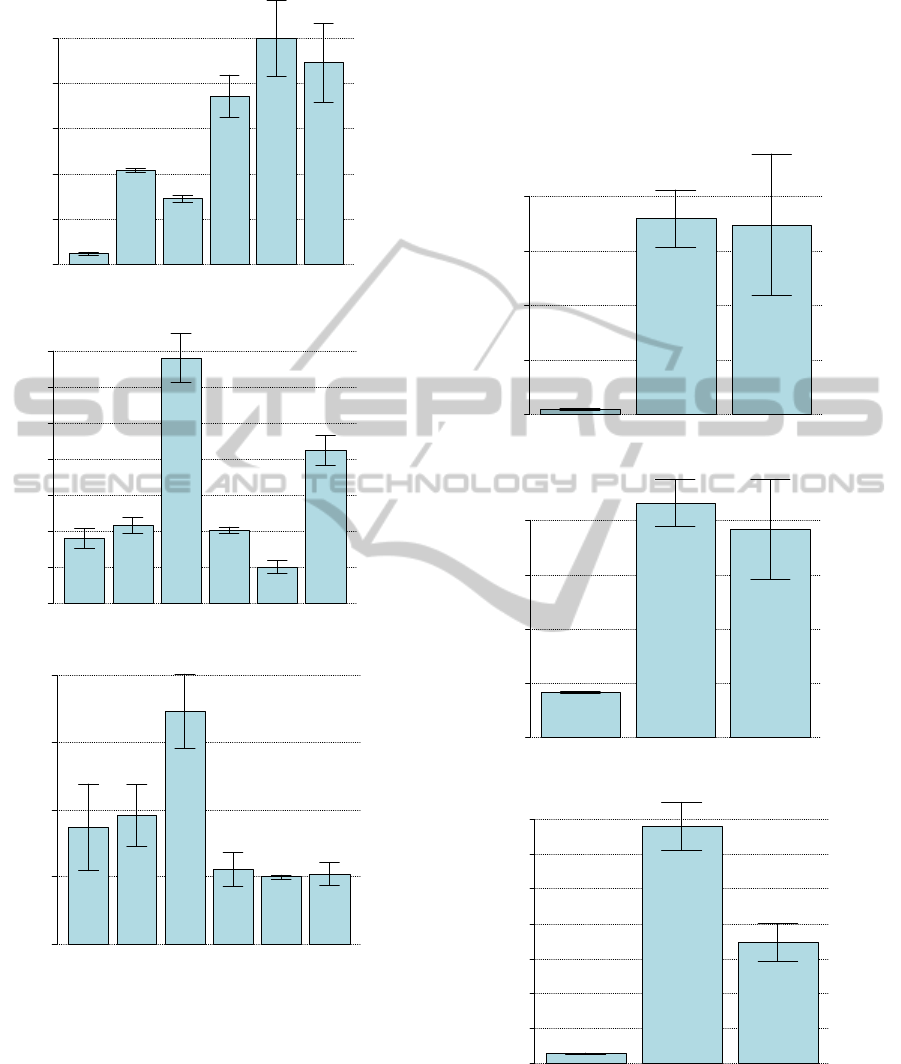
Figure 1: Expression levels of GOI1, GOI2 and GOI3,
respectively, in control (Col0) and mutant (M) and after
treatments (0h, 2h, 4h). Error bars represent the standard
deviation for each biological condition.
3.2 Comparison between Samples
Figure 2 plots respectively all three GOI in the
biological conditions Col0h1, Col2h1 and Col4h1
with their associated standard deviations. Similarly,
Figure 3 plots the GOIs in the biological conditions
M0h1, M2h1 and M4h1, respectively. An example
of pairwise comparisons statistical analysis is
provided in Table 2. We have highlighted all
significantly different pair-wise comparisons in bold
of Table 2.
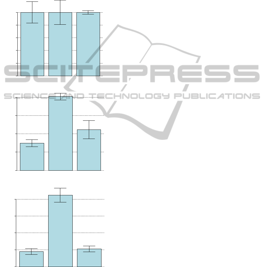
Figure 2: Expression of GOI in each treatments.
Expression levels of GOI1, GOI2 and GOI3, respectively,
in each condition treatment col0h1, col2h1, col4h1,
respectively. Error bars represent the standard deviation
for each condition.
Expression of gene GOI1
0.0 0.2 0.4 0.6 0.8 1.0
col0h1
col2h1
col4h1
M0h1
M2h1
M4h1
Expression of gene GOI2
01234567
col0h1
col2h1
col4h1
M0h1
M2h1
M4h1
Expression of gene GOI3
01234
col0h1
col2h1
col4h1
M0h1
M2h1
M4h1
Expression of genes in sample col0h1
0.0 0.5 1.0 1.5 2.0
GOI1
GOI2
GOI3
Expression of genes in sample col2h1
0.0 0.5 1.0 1.5 2.0
GOI1
GOI2
GOI3
Expression of genes in sample col4h1
01234567
GOI1
GOI2
GOI3
BIOINFORMATICS2013-InternationalConferenceonBioinformaticsModels,MethodsandAlgorithms
206

Table 2: Presentation of statistical results for GOI1, GOI2 and GOI3, respectively. pvalue inferior to 5% is in bold.
GOI1
Sample col0h1 col2h1 col4h1 M0h1 M2h1 M4h1
col0h1 1,000
0,002 0,004 0,002 0,002 0,004
col2h1 NA 1,000
0,024
0,109 0,068 0,154
col4h1 NA NA 1,000
0,030 0,024 0,054
M0h1 NA NA NA 1,000 0,559 0,818
M2h1 NA NA NA NA 1,000 0,772
M4h1 NA NA NA NA NA 1,000
GOI2
Sample col0h1 col2h1 col4h1 M0h1 M2h1 M4h1
col0h1 1,000 0,584
0,015
0,557 0,228 0,053
col2h1 NA 1,000
0,018
0,917 0,115 0,080
col4h1 NA NA 1,000
0,005 0,008
0,150
M0h1 NA NA NA 1,000 0,089
0,026
M2h1 NA NA NA NA 1,000
0,018
M4h1 NA NA NA NA NA 1,000
GOI3
Sample col0h1 col2h1 col4h1 M0h1 M2h1 M4h1
col0h1 1,000 0,820 0,239 0,998 0,841 0,909
col2h1 NA 1,000 0,334 0,790 0,905 0,853
col4h1 NA NA 1,000 0,122
0,020
0,062
M0h1 NA NA NA 1,000 0,768 0,878
M2h1 NA NA NA NA 1,000 0,846
M4h1 NA NA NA NA NA 1,000
GOI1 is induced in Col plants by a factor of forty 2h
after wounding and by a factor of thirty 4h after
wounding (pvalue= 3.9.10
-5
and 2.10
-4
, respectively).
We also observed a 4-fold induction of GOI2
(CYP76C5) in Col plants 4h after wounding
(pvalue=0.0015). GOI2 is also significantly
differentially expressed between Col and M 4h after
wounding (pvalue=0.0288).
In Figures 2 and 3 we have summarized the
results of GOI1 compared to the two other GOIs
including statistical pair-wise comparisons using t-
tests in all conditions studied. Expression of GOI1 in
Col0h is statistically different from all the other
conditions studied: wounding in both Col and
mutant as well as control mutant (t=0h). GOI2 is
induced more than 3-times 4h after wounding in Col
plants (pvalue=0.0015) compared to Col plants
without wounding.
4 DISCUSSION
The data analyzed here as an example include only a
small set of genes and biological conditions but the
R-script does not have a limit on the number of
samples and genes that can be included. Our method
includes the option for biological data in addition to
technical replicates. The biological replicates were
not taken in account in the qBASE software
however they are very important in the design of
meaningful biological experiments. The second
difference in our script compared to qBASE is the
absence of inter-run control in our script but it can
be implemented for diagnostic validated by qPCR.
The use of normalization was also available in the
functions “relQuantPCR” and “normPCR” in the
SLqPCR package as we propose it in formula 2 and
4. Another very important feature included in our R-
RqPCRAnalysis:AnalysisofQuantitativeReal-timePCRData
207
script is the statistical validation of the results for the
biologist. The principle statistical validation of the
results we describe in formula 14 was available in
the HTqPCR package but done on Cq values
(Dvinge and Bertone, 2009) and in the web-based
QPCR (Pabinger et al., 2009).
Figure 3: Expression of GOI in each treatment. Expression
levels of GOI1, GOI2 and GOI3, respectively, in each
condition treatment M0h1, M2h1, M4h1, respectively.
Error bars represent the standard deviation for each
condition.
Finally our R-script program can be used with
any qPCR machine softwares since a simple text file
is necessary as the input file. The qpcR package is
also using the error propagation formula we use in
formula 7 however the “ratiocalc” function is used
on raw Cq value and on efficiency values rather than
on normalized expression value as we do in our
package.
The biological condition determines as the
reference condition (value 1) is chosen by the
biologist. Our program also allows the modification
of the figures in any graphic software in order to
personalize the colour, legends, x- or y-scale for
instance.
The R-script described in this paper implements
features for qPCR analysis that are scattered in
several packages, or available in commercial
packages.
Our data demonstrated the over-expression of
GOI1 in our mutant plants as well as induction of its
expression in Col and mutant plants after mechanical
wounding. The expression of GOI2 is also
modulated according to plant genotypes in the time
course of the wounding. The last gene studied in our
experiment, GOI3, did not show any statistically
valid repression or induction in all conditions
described in our experiment.
5 CONCLUSIONS
We have presented in this paper a free R-script
program that can be easily used by biologists and
that is independent of the qPCR instrument software.
Our script includes:
-Biological replicates in the design of the experiment
as well as technical replicates
-The choice of reference genes using Genorm
formulas (Vandesompele et al., 2002),
-The normalization and rescaling of expression
levels for each GOI using qBASE software formulas
(Hellemans et al., 2007),
-A flexible graphic representation of gene
expression levels including standard deviations
-Statistical tests to validate the differentially
expressed genes compared to controls.
This software is user-friendly for biologists and a
step by step guide is available. It was already used in
two publications (Brun et al., 2010); (del Giudice et
al., 2011); (Giraudo et al., 2011).
Expression of genes in sample M2h1
0.0 0.2 0.4 0.6 0.8 1.0
GOI1
GOI2
GOI3
Expression of genes in sample M0h1
0.0 0.5 1.0 1.5 2.0
GOI1
GOI2
GOI3
Expression of genes in sample M4h1
01234
GOI1
GOI2
GOI3
BIOINFORMATICS2013-InternationalConferenceonBioinformaticsModels,MethodsandAlgorithms
208

ACKNOWLEDGEMENTS
This work was supported by an Agence Nationale de
la Recherche Grant 06 BLAN 0346 given to R.
Feyereisen, UMR IBSV INRA-CNRS-Université de
Nice Sophia Antipolis. The authors thank R.
Feyereisen and E. Wanjberg for useful discussion
and correction of the manuscript. Trang Tran was
financially supported by an Agence Nationale de la
Recherche Grant 06 BLAN 0346 given to R.
Feyereisen.
REFERENCES
Brun-Barale, A., Héma, O., Martin, T., Suraporn, S.,
Audant, P., Sezutsu, H., Feyereisen, R., 2010 Multiple
P450 genes overexpressed in deltamethrin-resistant
strains of Helicoverpa armigera, Pest Management
Science, 66: 900-909.
Bustin, S. A., 2002. Quantification of mRNA using real
time reverse transcription PCR ( RT-PCR): trends and
problems. Journal of Molecular Endocrinology, 29:
23-39.
Bustin, S. A., 2004. A-Z of Quantitative PCR. La Jolla
California: International University Line.
Bustin, S. A., Benes, V., Garson, J. A., Hellemans, J.,
Huggett, J., Kubista, M., Mueller, R., Nolan, T., Pfaffl,
M. W., Shipley, G. L., Vandesompele, J. and Wittwer,
C. T., 2009. The MIQE Guidelines: Minimum
Information for Publication of Quantitative Real-Time
PCR Experiments. Clinical Chemistry, 55 (4): 611-
622.
Bustin, S. A., Beaulieu, J.-F., Huggett, J., Jaggi, R.,
Kibenge, F., Olsvik, P., Penning, L. and Toegel, S.,
2010. MIQE precis: Practical implementation of
minimum standard guidelines for fluorescence-based
quantitative real-time PCR experiments. BMC
Molecular Biology, 11 (74).
Czechowski, T., Bari, R.P., Stitt, M., Scheible, W.-R. and
Udvardi, M.K., 2004. Real-time RT-PCR profiling of
over 1400 Arabidopsis transcription factors:
unprecedented sensitivity reveals novel root- and
shoot-specific genes. Plant Journal, 38: 366-379.
del Giudice, J., Cam, Y., Damiani, I., Fung-Chat, F.,
Meilhoc, E., Bruand, C., Brouquisse, R., Puppo, A.
and Boscari, A., 2011. Nitric oxide is required for an
optimal establishment of the Medicago truncatula-
Sinorhizobium meliloti symbiosis. New Phytologist,
190.
Giraudo, M., Califano, J., Hilliou, F., Tran, T., Taquet, N.,
Feyereisen, René, Le Goff, G., 2011. Effects of
Hormone Agonists on Sf9 Cells, Proliferation and Cell
Cycle Arrest. PLoS ONE, 6, 10, e25708.
Dvinge, H. and Bertone, P., 2009. HTqPCR: High-
throughput analysis and visualization of quantitative
real-time PCRdata in R. Bioinformatics, 25, 3325-
3326.
Hellemans, J., Mortier, G., De Paepe, A., Speleman, F.
and Vandesompele, J., 2007. qBase relative
quantification framework and software for
management and automated analysis of real-time
quantitative PCR data. Genome Biology , 8 (2):R19.
Pabinger, S., Thallinger, G., Snajder, R., Eichhorn, H.,
Rader, R. and Trajanoski, Z., 2009. QPCR:
Application for real-time PCR data management and
analysis. BMC Bioinformatic, 10, 268.
Park, J.-H., Halitschke, R., Kim, H. B., Baldwin, I. T.,
Feldmann, K.A. and Feyereisen, R., 2002. A knock-
out mutation in allene oxide synthase results in male
sterility and defective wound signal transduction in
Arabidopsis due to a block in jasmonic acid
biosynthesis. Plant Journal, 31: 1-12.
Vandesompele, J., De Preter, K., Pattyn, F., Poppe, B.,
Van Roy, N., De Paepe, A. and Speleman, F., 2002.
Accurate normalization of real-time quantitative RT-
PCR data by geometric averaging of multiple internal
control genes.
Genome Biology, 3.
APPENDIX
Demonstration of RqPCRAnalysis Package
R-script
The package RqPCRAnalysis will be submitted to
Bioconductor (http://www.bioconductor.org).
RqPCRAnalysis is one of a default set of packages
installed by biocLite in the Bioconductor project.
The core Bioconductor packages can be installed
from the command line of R.
We assume that an experiment has been
conducted with one or more biological replications
and each sample has one or more technical
replicates. The data are stored in ".txt" file and have
the following table structure (recommended). Note
that the biological replicates must be ranked
successively by different blocks. The suffix _j is
recommended to distinguish the biological replicate.
In each block of biological replicates, the technical
replicates of each sample are also ranked
successively in sub-block "pair by pair" (Table 2).
"Efficiency" is the PCR amplification efficiency
coefficient established for each qPCR array (i.e.
each primer couple) by means of calibration curves.
This coefficient should be determined from the slope
of the log-linear portion of the calibration curve.
Specifically,
10
1
(16)
when the logarithm of the initial template
concentration is plotted on the x-axis and Cq is
plotted on the y-axis (4)
RqPCRAnalysis:AnalysisofQuantitativeReal-timePCRData
209

In the beginning, one computes all parameters
for each gene in each biological block: Mean.Cq
(Mean of Cq), SD.Cq (Standard Deviation of Cq),
QCq (Relative Quantity) and SD.QCq (Standard
Deviation of QCq). See Section Statistical methods
for detail.
Validation Reference Genes
The reference genes (REF), previously referred as
housekeeping gene is then selected. By default a
function of the script [select.ref.genes()] provides a
list of REF by finding the most stable genes (at least
2) across all biological replicates. Otherwise REF
can be chosen manually (not recommended). The
[select.ref.genes()] function ranked the genes from
most stable to least stable as done in (5).
qPCR Data Analysis and Graph Representations
The normalization factor based on these REFs for
each gene of interest (GOI) is then computed. The
normalised expression consists of the expression
level, as well as the standard deviation and the
standard error associated for each biological
replicates. As a convention, this function applies for
each biological replicate. Rescaling the normalized
expression for each GOI is done according to
qBASE (5) and our script is able to run with missing
values at this step.
Statistical Studies of Gene Expressions
Our script then provides sample comparisons which
were not included in qBASE. Here we use the
method of pair-wise t-tests. For each GOI, all pairs
of samples across biological replicates are
compared. The normalized expression output or the
rescaled expression output can be tested. Graphs of
the results are available to export, they contain
normalized expression or rescaled expression and
the GOI to be plotted can be chosen. By default all
the GOI will be represented on the graph with their
standard deviations but representation with standard
errors can be plotted as well. In complement to the
graphs, a table is given containing the rescaled
expression values as well as their corresponding
standard deviation. An additional table with the
results of pair-wise comparison using t-tests is also
provided.
Data Import
We assume that an experiment has been conducted
with one or more biological replications and each
sample has one or more technical replicates. The
data are stored in .TXT file and have the following
Table 3 (recommended). Note that the biological
replicates must be ranked successively by different
blocks. The suffix _j is recommended to distinguish
the biological replicate. In each block of biological
replicates, the technical replicates of each sample are
also ranked successively in sub-block "pair by pair"
(see the example file "example.txt"). "Efficiency" is
the PCR amplification efficiency coefficient
established for each qPCR array (i.e. each primer
couple) by means of calibration curves. This
coefficient should be determined from the slope of
the log-linear portion of the calibration curve (2).
Table 3: Data storage format.
Sample Gene1 Gene2
efficiency 2 1.8
Biologic
al replicate 1
Sample1_1 23 25
Sample1_1 24 30
… … …
Samplei_1 21 10
Samplei_1 11 12
Biologic
al replicate j
Sample1_j 12 12
Sample1_j 14 15
… … …
Samplei_j 21 22
Samplei_j 25 23
Biologic
al replicate m
Sample1_
m
14 17
Sample1_
m
21 25
… … …
Samplei_
m
14 15
Samplei_
m
12 14
Data Analysis
- Reading data into workspace:
> data <-
read.data(filename="example.txt",pa
th=path,bio.rep=3)
Computing parameters for each biological
replicates:
> parameter<-
pcr.processing(data,num.rep=2,na.rm
=TRUE)
- Computing normalisation factor: Finding most
stablity genes (REF) and normalization factor based
on REF:
> stability.value<-
reference.genes(data, num.ref = 3,
na.rm = TRUE)
> ref.gene<-
as.character(stability.value$order[
1:3])
BIOINFORMATICS2013-InternationalConferenceonBioinformaticsModels,MethodsandAlgorithms
210

(or > ref.gene<-
c("REF1","REF2","REF3")
> ref.factor <-
normalization.factor(parameter,ref.
gene=ref.gene)
- Computing expression level (normalized
expression) of genes of interest (GOI) in each
biological replicate based on normalization factor:
>normalized.exp<-
normalized.expression(parameter,ref
.factor,num.rep=2,
ref.gene=ref.gene,goi.gene=NULL)
- Comparing the difference
between samples across biological
replicates:
> comparison<-
test.sign(normalized.exp,bio.rep=3,
path=path)
- Computing the expression
across all biological replacates
for each gene:
> average<-
average.expression(normalized.exp,b
io.rep=3,na.rm = TRUE)
- Rescaling the normalized
expression for each GOI:
> final.result<-
rescaled.expression(average,na.rm =
TRUE)
- Plotting and saving results:
>pcr.plot(final.result,path=path
,goi.gene=NULL,sample.name=NULL,typ
e="gene",error="SE")
>qPCR.plot(final.result,path=pat
h,goi.gene=NULL,sample.name=NULL,ty
pe="sample",error="SE")
>
save.expression(final.result,path=p
ath,gene.names=NULL)
RqPCRAnalysis:AnalysisofQuantitativeReal-timePCRData
211
