Accurate Online Estimation of Battery Lifetime for Wireless Sensors

Network

Emmanuel Nataf

1,2

and Olivier Festor

Lorraine University, Vandoeuvre-l`es-Nancy, France

INRIA - MADYNES - Loria, Vandoeuvre-l`es-Nancy, France

Keywords:

Wireless Sensors Network, Energy Measurment, Battery lifetime, WSN430, Sky, Contiki, Cooja.

Abstract:

Battery is a major hardware component of every device in a wireless sensor network. Most of them have no

power supply and are generally deployed for a long time. Investigations have been done on battery physical

models and their adaptation to sensors. We present an adaptation and instanciation of such a model on a real

sensor operating system and how architectural constraints have been considered. Experiments have been made

in order to test the impact of several parameters on the battery lifetime.

1 INTRODUCTION

Wireless Sensors Networks (WSN) have a growing

presence in industrial and home automation. These

constrained networks are made possible by the reduc-

tion of processor size and the high performance bat-

teries. Nevertheless these networks have to take care

of their energy consumption because they are usually

deployed for a long time. The growing interest on bat-

tery lifetime estimation for WSN appears in the stan-

dardization work of these network (Ed., 2012). They

deﬁne a routing protocol with one metric being the

remaining battery level (Vasseur Ed. et al., 2012).

Battery models that describe relation between the

battery lifetime and its use have been proposed since

embedded systems (laptop, cellular phone) became

popular. These models take into account two phe-

nomenons occurring in a battery cell: the Rate Ca-

pacity Effect and the Recovery Effect (Panigrahi et al.,

2001). The former gives the energy consumed under

a constant current load, when transmitting for exam-

ple, and the latter gives the energy recovered during

inactivity or low current load. Inside a battery, oxi-

dation at the anode electrode induces reduction at the

cathode. The reduction decreases the concentration

of positive ions near the cathode and so the available

energy. But during idle time or low current load posi-

tive ions near the anode have time to move toward the

cathode, thus increasing the available energy and so

the battery lifetime.

The analytical model of this battery behaviour is

well known but is too complex to be instanciated on

a sensor board. However, an approximation of this

model is available and our contribution in this paper

is to ﬁll the last gap between the approximated model

and its instanciation within an existing operating sys-

tem for sensors. The remainder of this paper is orga-

nized as follow. We ﬁrst describe the reference model

and its approximation. The next section emphasizes

on the elementary operations of WSN node and their

current draw. Details of the implementation are given

in the section 4 and ﬁrst results are shown in the last

part. We draw some conclusions and forecast future

work at the end of the document.

2 REFERENCE MODEL

The most accurate battery modeling is given by the

analytical equation (1) (Rakhmatov and Vrudhula,

2001; Rakhmatov et al., 2002; Rao et al., 2003). In

this formula, α (coulombs) denotes the total battery

capacity that is equals to the current load i(τ) – in the

left additive operand – consumed since the use of the

battery until the time L (the battery Lifetime) and –

the second operand – the current that was unavailable

because positive ion concentration was not sufﬁcient

at the cathode. The β parameter is the diffusion coef-

ﬁcient of electroactive species inside the battery. β

expressed in s

−1

α =

i(τ)dτ + 2

∞

∑

m=1

i(τ)e

−β

(L−τ)

dτ (1)

Nataf E. and Festor O..

Accurate Online Estimation of Battery Lifetime for Wireless Sensors Network.

DOI: 10.5220/0004312500590064

In Proceedings of the 2nd International Conference on Sensor Networks (SENSORNETS-2013), pages 59-64

ISBN: 978-989-8565-45-7

 2013 SCITEPRESS (Science and Technology Publications, Lda.)

The use of this model can be found in (Rakhmatov

and Vrudhula, 2003; Seungki et al., 2005; Timmer-

mann, 2003; Zhang et al., 2010; Sausen et al., 2010)

for various domains, as task scheduling or simulation.

The model can not be implemented as is on WSN

nodes albeit some results with the ﬁrst part of equa-

tion (1) are reported in (Dunkels et al., 2007; Kera-

siotis et al., 2010). In so doing, no work does to our

knowledge take into account the recovery effect that

occurs during idle time despite it is generally more

than 90% of the WSN node lifetime. The contribu-

tion of (Rahm´e et al., 2010) is an approximation of

equation (1) that can be implemented on WSN node.

The global equation (2) recursively computes σ(L

)

that is the consumed charge in Milli ampere minute

(mAmn) at time L

. This computation depends on the

consumed charge at time L

n−1

, the time interval, in

minute, ∆ = L

−L

n−1

being constant.

σ(L

) =

∑

k=1

+ λ

σ(L

n−1

) −

n−1

∑

k=1

+2I

A(L

n−1

+ δ

n−1

)

(2)

With this approach, we know the remaining charge

in the battery at time L

by the difference between

σ(L

) and the initial battery parameter α of equation

(1). The recovery effect of the battery is computed

through the function A given in the equation (3) that

is approximated by the use of an f function we detail

below.

A(L

n−1

+ δ

n−1

) =

∞

∑

m=1

−β

−L

n−1

−δ

)

−e

−β

−L

n−1

)

≃

f(ν)

−

f(∆)

(3)

This approximation depends on the idle time of the

mote during the ∆ interval, given by the difference

ν = ∆ −δ

(ν is the idle time of the L

n−1

period

and δ

its activity time). The recursivity of the

model depends on the λ parameter deﬁned as the ratio

A(L

n+1

,δ

,0)

A(L

,δ

,0)

for each n but that can be bounded by the

value e

−β

∆

computed ofﬂine.

3 CURRENT DRAW

3.1 Linear Draw

The ﬁrst term in equation (2) is the sum of products

between current load I

and time interval δ

since the

beginning of the battery lifetime (when k = 1) un-

til the time L

. The δ

time interval is a sub inter-

val of ∆ during which the battery was used by the

node. To compute this value we must know which

components of the motes use the current along the

time and at which current rate. Mote’s current infor-

mation can be obtained from data-sheet documents.

For example, the table 1 shows the current load for

two mote types (Sky or WSN430 motherboard, re-

spectively with CC2420 and CC1100 communica-

tion chips). The columns are the usual states of the

duty cycle for any mote : CPU, LPM, TX and RX

respectively for processor, low power mode, trans-

mitting and receiving. Currents are given in mA.

The given values for TX and RX are linked to sig-

nal power and throughput conﬁguration of the mote.

We have launched experiments on the senslab plat-

Table 1: Motes current draw.

Mote CPU LPM TX RX

Sky 1.8 0.0545 17.4 18.8

Wsn430 2 0.02 16.1 15.2

form (des Roziers et al., 2011) with one tested node

(WSN430 based). The senslab testbed provides an

external polling service of the current consumed by

motes during an experiment. We program the node to

print the time of each state change. The ﬁgure 1 shows

17 17.5 18 18.5 19 19.5 20

Current (mA)

Time (s)

external

Figure 1: Mote modes and currents.

plots of measured current at the mote endpoints and

the duties cycles (we just keep TX and RX mode that

have the main current values). Note that start and stop

times of duties match with measured current. Conse-

quently, the current draw of a ∆ = δ

CPU

+ δ

LPM

inter-

val is the result of the equation (4) where eachC

state

the current load (cf.table 1) and each δ

state

is the sum

of all state sub-intervals inside ∆.

= C

CPU

.δ

CPU

LPM

.δ

LPM

.δ

(4)

SENSORNETS2013-2ndInternationalConferenceonSensorNetworks

4 IMPLEMENTATION

CONSTRAINTS

Even with the help of (Rahm´e et al., 2010), we must

be aware of mote limitations on code size and arith-

metical capabilities. The strong constraint is that the

MSP430 compiler can not handle ﬂoating point val-

ues but only signed or unsigned integer.

4.1 Online Computation

We compute the consumed current every ∆ time inter-

val. The values δ

CPU,LPM,TX,RX

are provided in Milli

second and we use the current load of the table 1 with

a factor of thousand. The result’s unit is in µA.ms then

it is converted in mA.mn (cf eq. (2)). We compute ν

with the low power mode period and the radio use :

ν =



LPM

−(δ

+ δ

) if δ

LPM

> (δ

+ δ

)

0 else

(5)

If the radio is more used than the LPM state then there

is no idle time for the battery. The varying part of the

recovery function A (equation 3) is rewritten in order

to lose as little precision as possible :

f(ν)

ν+ π

2.10

−12β

√

12.10

(6)

At this step we use a 64 bits intermediary value to get

the result (MSP430 compiler allows such data type

but they are actually emulated with several 32 bits val-

ues).

Finally, the remaining energy is computed with

the values above and the previous remaining energy

value (a ∆ before). We compute the ratio with 255

as 100%. This value is given by a WSN routing met-

ric recommendation (Vasseur Ed. et al., 2012) and

we use it in the present work to implement and test an

energy-based routing plane. However we compute the

remaining energy with a precision of 5 numbers, that

is from 255.10

, so energy consumption is measured

at a very ﬁne granularity.

The code size of the presented implementation is

about 12Kb out of the 50Kb allowed by our sensor

board. At the memory level, we store on memory

six 32 bits values from one computation to the other

(times of CPU, LPM, TX, RX and previous values for

σ(L

n−1

) and

∑

n−1

k=1

5 SIMULATION RESULTS

For our simulations we use the Cooja WSN simulator

(Osterlind et al., 2006) and test a network of nodes

built on the Sky mote platform. All node have an ini-

tial battery charge of 880mAh, that give a value for α

of 880 = 52800mAmn because we consider an ideal

battery for these ﬁrst steps. For the same reason, we

choose the value β = 1.

Nodes use IPv6 and the RPL

routing protocol

(Ed., 2012) to perform a simple collect application

during which one or more nodes, the Senders, pe-

riodically send sensing information to a receiving

node called the Sink, conﬁgured to be the root of the

RPL routing tree. Senders send one data packet ev-

ery second and use the contikiMAC radio duty cycle

(Dunkels, 2011). We use a linux Ubuntu 11.0 desk-

top computer with a 3GHz Intel processor and 4Gb of

memory to run simulations.

5.1 Booting Node

We start our experiment with the observation of the

node booting process. The ﬁgure 2 puts together the

evolution of the battery lifetime and the time spends

by activities of the node. During the ﬁrst minute, on

the part (a), we note a large decrease of the battery

correlate with the strong activity on the part (b) for the

same period. Mainly this activity is related to system

and network initialization (remains the strong power

for TX and RX of the table 1). The battery recovery

is visible at this very detailed level, during the second

minute and the two following ones. These recovery

periods match with low activity periods.

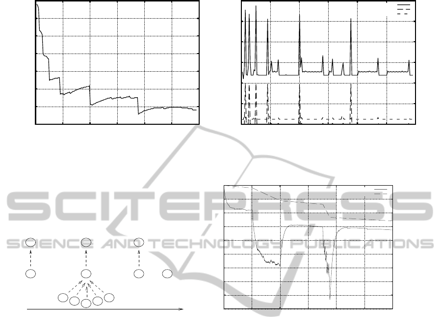
5.2 Network Building

We continue the simulation shown in the ﬁgure 3 (a)

where after ten minutes of simulated time, we add

ﬁve nodes “under” the non-root node to observe the

cost of the routing tree building and trafﬁc accumula-

tion. The node 1 is the Sink and all other are Sender.

We leave these nodes sending and forwarding (only

for the node 2) data packets during ten minutes and

remove the ﬁve nodes previously added. This can

occurs in real deployement for example with mobile

nodes or with lossy communication environment. A

ﬁnal point of interest, at the thirty ﬁfth minute, is

when a node has lost its destination node (its default

next hop router) because the network has to build it-

self again. The ﬁgure 3(b) plots the remaining bat-

tery lifetime of the node 2 along our experiment. The

recovery

curve is related to the implementation and

the

linear

is a simple additive function of current

draw. The strong decrease of the ﬁrst ten minutes is

mainly due to trafﬁc overhead and very few is from

Routing Protocol for Low-Power and Lossy Network

that is only 0.0005% of the total

AccurateOnlineEstimationofBatteryLifetimeforWirelessSensorsNetwork

99.9993

99.9994

99.9995

99.9996

99.9997

99.9998

99.9999

100

0 1 2 3 4 5 6

Battery lifetime (%)

Time (mn)

100

150

200

250

300

0 1 2 3 4 5 6

Duties schedule (ms)

Time (mn)

CPU

(a) (b)

Figure 2: First minutes of battery lifetime.

4 6

3 7

2 2

Time (mn)

0 10 20 35

99.55

99.6

99.65

99.7

99.75

99.8

99.85

99.9

99.95

100

0 10 20 30 40 50 60

Battery lifetime (%)

Time (mn)

recovery

linear

(a) (b)

Figure 3: Battery lifetime and RPL.

RPL control messages. Once the routing plane is es-

tablished, between the tenth and twentieth minute, the

battery decreases with a greater slope and with more

micro variations. When removing nodes at the twen-

tieth minute, the node 2 shows a quick and strong re-

covery of its battery lifetime. As given by the model,

the fall of current draw lets the battery recovers some

of its current charge. During the ﬁfteen following

minutes the node sends one packet per second to the

Sink and the curve is similar to the beginning (with-

out booting process) but at a lower battery level. At

the thirty ﬁfth minute we remove the parent of the

node 2. The very large decrease of battery is again

mainly related to a strong use of communication. The

node has no more IPv6 router neighbor then it polls

the network with neighbor discovery messages and

after three minutes, the node decides to build a new

network and just send few RPL control message. One

can there observe a very signiﬁcant recovery at the

part (b). The linear model is very less reactive and

never grows, as expected. It generally over estimates

the lifetime and it does not take into account the re-

covery effect.

5.3 Radio Duty Cycle

The Contiki operating system supports some RDC

implementations we have used in order to compare

their energy consumption. The part (a) of ﬁgure 4

shows these experiments. All these RDC are asyn-

chronous and packet oriented.

• the contikiMAC allows the greatest battery life-

time. It can sleep up to 99% of the time and was

measured as been ten times less energy consumer

than X-MAC (Dunkels, 2011).

• X-MAC (Buettner et al., 2006) is a bigger con-

sumer; the sender sends several preamble packets

until an acknowledge reception and then sends the

data packet.

• CX-MAC (Compatibility X-MAC) is a variation

of X-MAC that is provided by Contiki to be usable

on more radio chips.

SENSORNETS2013-2ndInternationalConferenceonSensorNetworks

100

0 5 10 15 20 25 30

Battery lifetime (%)

Time (day)

contikiMAC

X-MACCX-MACsicslowMAC

100

0 5 10 15 20 25 30

Battery lifetime (%)

Time (day)

(a) (b)

Figure 4: Network life.

• sicslowMAC (also in Contiki) handles 802.15.4

frames and always keeps its radio open.

As one can expect, RDC has a strong effect on the

battery lifetime and this effect is mainly due to the

use of radio of each RDC.

5.4 Throughput

We have also measured the throughput effect on bat-

tery lifetime and plot them in part (b) of the ﬁgure

4. The contikiMAC RDC was used because it is the

less battery consuming stack and so the impact of

the throughput is emphasized. Numbers within the

part (b) are the throughput of the application, from 60

packets by minute (pkts/mn) to 1. Each packet has a

size around 100 bytes and the application is parame-

terized by a number of seconds between two packets.

These results show that the lifetime is roughly linear

with the throughput but other tests with less through-

put than 1pkt/mn have no signiﬁcant improvement

on the lifetime. The network trafﬁc is then negligible

compared to sensor base activity (indeed the routing

protocol is the main radio consumer).

5.4.1 Lifetime Estimation

These ﬁgures are very close to a line and we use a

linear regression with the least square estimation tech-

nique to envisionthe time when the battery is depleted

(i.e. with 0% of remaining energy). Table 2 contains

the battery lifetime estimation for each lines in ﬁgure

4. The short lifetimes of these networks (no more than

four months) is related to the light battery we have

used. Battery of node like Sky are usually around

2000mAh and should allow WSN be operational for

one year. Nevertheless real batteries have a secure cut

off level that prevent them to be fully discharged be-

cause they will be damaged and not able to be charged

again.

Table 2: Battery life estimation.

RDC Lifetime

(days)

contikiMAC 128

X-MAC 30

CX-MAC 26

sicslowMAC 1.8

Thgput : 1pkt/mn

Thput Lifetime

(pkts/mn) (days)

60 77

20 105

12 113

2 124

RDC : contikiMAC

6 CONCLUSIONS

We presented a ﬁrst implementation of a battery life-

time estimation inside an existing operating system

for WSNs. Based on a recognized theoretical battery

model, our work has shown how the sensor internal

architecture impacts concrete realizations. Our simu-

lations help us to better understand how sensors use

their battery in the bootstrap process or during steady

networking phase. This work is useful for many ap-

plications like routing optimization that we currently

plan. The necessary additional work is to get the im-

plemented model and the real world closer tied. Dis-

charge tests of batteries must be done as precisely

as possible (manufacturer data-sheets are not always

enough) to parameterize the α and β values of the bat-

tery used. Such tests should be done at several ambi-

ent temperature level because it is know that it acts

on battery lifetime. The sensing chips (temperature,

light...) are also current consumer and some sensors

have energy scavenging capabilities that should be in-

tegrated into the model. We have to launch long time

testing (few weeks, months, one year) establishing a

AccurateOnlineEstimationofBatteryLifetimeforWirelessSensorsNetwork

relation between the remaining energy and the cut off

level of a battery. Moreover several battery technolo-

gies have to be tested to enforce our implementation

model.

REFERENCES

Buettner, M., Yee, G. V., Anderson, E., and Han, R. (2006).

X-mac: a short preamble mac protocol for duty-cycled

wireless sensor networks. In Proceedings of the 4th in-

ternational conference on Embedded networked sen-

sor systems, SenSys ’06, pages 307–320, New York,

NY, USA. ACM.

des Roziers, C., Chelius, G., Ducrocq, T., Fleury, E.,

Fraboulet, A., Gallais, A., Mitton, N., Noel, T.,

Valentin, E., and Vandaele, J. (2011). Two demos us-

ing senslab: Very large scale open wsn testbed. In In-

ternational Conference on Distributed Computing in

Sensor Systems and Workshops (DCOSS), pages 1–2.

Dunkels, A. (2011). The contikimac radio duty cycling pro-

tocol. SICS Technical Report T2011:13 ISSN 1100-

3154, Swedish Institute of Computer Science.

Dunkels, A., Osterlind, F., Tsiftes, N., and He, Z. (2007).

Software-based on-line energy estimation for sensor

nodes. In Proceedings of the 4th workshop on Em-

bedded networked sensors, EmNets ’07, pages 28–32,

New York, NY, USA. ACM.

Ed., T. W. (2012). Rpl: Ipv6 routing protocol for low-power

and lossy networks. RFC 6550, Internet Engineering

Task Force.

Kerasiotis, F., Prayati, A., Antonopoulos, C., Koulamas, C.,

and Papadopoulos, G. (2010). Battery lifetime predic-

tion model for a wsn platform. In Fourth International

Conference on Sensor Technologies and Applications

(SENSORCOMM), pages 525 – 530. IEEE.

Osterlind, F., Dunkels, A., Eriksson, J., Finne, N., and

Voigt, T. (2006). Cross-level sensor network simu-

lation with cooja. In Local Computer Networks, Pro-

ceedings 2006 31st IEEE Conference on, pages 641 –

648.

Panigrahi, D., Dey, S., Rao, R., Lahiri, K., Chiasserini, C.,

and Raghunathan, A. (2001). Battery life estimation

of mobile embedded systems. In Proceedings of the

The 14th International Conference on VLSI Design

(VLSID ’01), VLSID ’01, pages 57 – 63, Washington,

DC, USA. IEEE Computer Society.

Rahm´e, J., Fourty, N., Al Agha, K., and Van den Boss-

che, A. (2010). A recursive battery model for nodes

lifetime estimation in wireless sensor networks. In

Wireless Communications and Networking Confer-

ence (WCNC), pages 1 – 6. IEEE.

Rakhmatov, D. and Vrudhula, S. (2001). An analytical

high-level battery model for use in energy manage-

ment of portable electronic systems. In Computer

Aided Design, 2001. ICCAD 2001. IEEE/ACM Inter-

national Conference on, pages 488 – 493.

Rakhmatov, D. and Vrudhula, S. (2003). Energy manage-

ment for battery-powered embedded systems. ACM

Trans. Embed. Comput. Syst., 2(3):277–324.

Rakhmatov, D., Vrudhula, S., and Wallach, D. (2002). Bat-

tery lifetime prediction for energy-aware computing.

In Proceedings of the 2002 International Symposium

on Low Power Electronics and Design (ISLPED’02),

pages 154 – 159. ACM.

Rao, R., Vrudhula, S., and Rakhmatov, D. (2003). Battery

modeling for energy aware system design. Computer,

36(12):77 – 87.

Sausen, P. S., Spohn, M. A., and Perkusich, A. (2010).

Broadcast routing in wireless sensor networks with

dynamic power management and multi-coverage

backbones. Inf. Sci., 180(5):653–663.

Seungki, H., Daeyoung, K., and Jae-eon, K. (2005). Bat-

tery aware real time task scheduling in wireless sen-

sor networks. In 11th IEEE International Conference

on Embedded and Real-Time Computing Systems and

Applications, pages 269 – 272. IEEE.

Timmermann, D. (2003). Simulation of mobile wireless

networks with accurate modelling of non-linear bat-

tery effects. In In proceedings of Applied simulation

and modeling (ASM).

Vasseur Ed., P., Kim Ed., M., Pister, K., Dejean, N., and

Barthel, D. (2012). Routing metrics used for path cal-

culation in low-power and lossy networks. RFC 6551,

Internet Engineering Task Force.

Zhang, J., Ci, S., Sharif, H., and Alahmad, M. (2010). An

enhanced circuit-based model for single-cell battery.

In Applied Power Electronics Conference and Exposi-

tion (APEC), 2010 Twenty-Fifth Annual IEEE, pages

672 – 675.

SENSORNETS2013-2ndInternationalConferenceonSensorNetworks