
Inverse Modeling using a Wireless Sensor Network (WSN) for
Personalized Daylight Harvesting
Ryan Paulson
1
, Chandrayee Basu
1
, Alice M. Agogino
1
and Scott Poll
2
1
Berkeley Energy and Sustainable Technologies Lab, University of California at Berkeley, Berkeley, California U.S.A.
2
NASA Ames Research Center, Moffett Field, California, U.S.A.
Keywords: Intelligent Lighting Control, Wireless Sensor Network, Inverse Model, Predictive, Daylight Harvesting,
Piecewise Linear Regression, Building Energy Efficiency.
Abstract: Smart lighting systems in low energy commercial buildings can be expensive to implement and
commission. Studies have also shown that only 50% of these systems are used after installation, and those
used are not operated at full capacity due to inadequate commissioning and lack of personalization.
Wireless sensor networks (WSN) have great potential to enable personalized smart lighting systems for real-
time model predictive control of integrated smart building systems. In this paper we present a framework for
using a WSN to develop a real-time indoor lighting inverse model as a piecewise linear function of window
and artificial light levels, discretized by sub-hourly sun angles. Applied on two days of daylight and ten
days of artificial light data, this model was able to predict the light level at seven monitored workstations
with accuracy sufficient for daylight harvesting and lighting control around fixed work surfaces. The
reduced order model was also designed to be used for long term evaluation of energy and comfort
performance of the predictive control algorithms. This paper describes a WSN experiment from an
implementation at the Sustainability Base at NASA Ames, a living laboratory that offers opportunities to
test and validate information-centric smart building control systems.
1 INTRODUCTION
According to the U.S. DOE’s Energy yearbook in
2010, the maximum electricity consumption in
commercial buildings (13.6%) is attributed to
lighting (Department of Energy, 2010). Intelligent
daylight and occupancy-based lighting control is
becoming increasingly important for future net zero
energy buildings, for lighting as well as heating and
cooling energy savings. Fortunately, there have been
significant improvements in lighting controls and
associated hardware (Philips, 2011), in addition to
interoperability with building energy management
systems (Walton et al., 2007) and advances in
daylight harvesting systems such as smart windows
(Lee and Tavil, 2007); (Lu and Whitehouse, 2012).
Our prior work has demonstrated 50% savings
from individually dimmable and user preference-
based luminaire control in absence of daylight. An
additional 20% energy savings could be achieved
with daylight harvesting according to our simulation
results (Wen and Agogino, 2011a; 2011b); (Wen et
al., 2011); (Wen, 2008).
In spite of the growing impetus in lighting
control research and some successful pilot projects
(Lee and Tavil, 2007), the actual adoption of
intelligent lighting control systems in commercial
buildings has been very limited. Singhvi, Krause,
Guestrin, Garrett, and Matthews (2005) developed a
centralized lighting system to increase user comfort
and reduce energy costs by using a WSN. Suet Fei
Li (2006) developed wireless sensing and actuation
networks (WSAN) for lighting control in the home
environment. Lin and Megerian (2005) proposed a
decentralized algorithm for WSANs for optimal
lighting control.
Yet, as of 2010 70% of the US
national stock of commercial buildings had no
lighting controls for energy efficiency (Ashe et al.,
2012). Some of the reasons include general lack of
encouraging results of lighting retrofit in terms of
energy savings and system usability. Rude found
that 50% of the intelligent lighting control systems
they studied had been deactivated by the users and
the remaining 50% operated at 50% of target
performance (2006).
However, the drive to move to low energy and
213
Paulson R., Basu C., M. Agogino A. and Poll S..
Inverse Modeling using a Wireless Sensor Network (WSN) for Personalized Daylight Harvesting.
DOI: 10.5220/0004314302130221
In Proceedings of the 2nd International Conference on Sensor Networks (SENSORNETS-2013), pages 213-221
ISBN: 978-989-8565-45-7
Copyright
c
2013 SCITEPRESS (Science and Technology Publications, Lda.)

even net zero energy usage has led to more
buildings being retrofitted or commissioned with
automated control capabilities. A major challenge is
to control the coupled sub-systems of a complex
building system or even a cluster of buildings.
Moving beyond the capabilities of heuristic control
approaches, new systems seek to incorporate
predictive models of occupancy, renewable energy
availability and price signals (Ma et al., 2012); (Liu
and Henze, 2006) to account for interdependencies
between energy performance of these subsystems
(Mukherjee et al., 2010). The sub-system
interdependencies and their influences on the overall
building energy performance could be captured by
massive deployment of wireless sensor networks
(Brambley et al., 2005); (Lin and Megerian, 2005);
(Li, 2006) and real-time modelling.
Assuming an energy cost of 16.8 cents/kWh
(California Public Utilities Commission, 2011) and
an annual energy intensity of 131.0 to 177 kWh/m
2
(California Energy Commission [CEC], 2006), the
average annual energy cost of small and medium
commercial buildings in California is $30/m
2
; 29%
of this energy is used in commercial lighting (CEC,
2006). 50-60% lighting energy savings from daylight
harvesting and feedback lighting control would
therefore mean an energy cost savings of $5.20/m
2
per year. A scenario of 2 to 3 wireless sensor
platforms per workstation (Deru et al., 2011)
including daylight sensors, amounts to 1
platform/6.2 - 9.3 m
2
, the standard occupancy being
18.6m
2
/person, according to the standards for
ventilation set by the American Society of Heating,
Refrigerating, and Air-Conditioning Engineers
(ASHRAE) (ASHRAE, 2010). The current price of
most commercially available wireless sensor
platforms is approximately $100. Hence, the initial
investment for a WSAN-based closed loop lighting
control system is approximately $10.70-$16.00/m
2
(just for the sensor platform), which is 2-3 times
higher than the annual lighting energy cost per unit
area of a building.
Thus one major challenge is the development of
inexpensive and easy to commission WSANs, along
with computationally inexpensive lighting models
and intelligent control systems. The question is how
minimal sensor deployment could suffice for desired
energy and comfort performance of thesesystems.
One strategy is to repeatedly redeploy the same
wireless sensor platform in different locations at
desktop levels to create parameterized lighting
models. This redeployment promises to cut down
costs in comparison to sensors permanently fitted in
luminaires. This strategy also can increase accuracy,
as the overhead sensors tend to over-estimate the
light level compared to the human eye at desktop
levels. Sensor platform reuse can be facilitated by
inclusion of a predictive mathematical model of the
indoor light level at key locations (such as desktops)
within the intelligent lighting control loop, as a
function of the minimum required sensed data
points.
In this paper we present a framework for the
development of an indoor lighting inverse model as
a piecewise linear function of the minimum number
of sensed parameters: window light levels and
adjoining dimmable lights’ statuses, discretized by
sub-hourly sun angles at a given time of the day. As
part of our on-going research on information-centric
smart building control systems, we deployed low
power wireless light sensor network for system
identification at the Sustainability Base at the NASA
Ames Research Center. The training and validation
data for the predictive inverse lighting model were
obtained after three months of data acquisition at this
test bed.
2 ANALYSIS
2.1 Inverse Problem Theory
Inverse problem theory describes methods by which
a model of a system is developed by: (1)
parameterizing the system in terms of a set of model
parameters that adequately characterize the system
in the desired point of view, (2) making predictions
on the actual values based on physical laws and
given values of the model parameters, and (3) using
actual results from measurements to determine the
model parameters (Tarantola, 2005).
A physics-based lighting model is the best choice
for accuracy, requiring the input of accurate building
and furniture dimensions. These models estimate the
lighting as a summation of the luminaries and
daylight at every position in the room. These
systems can be difficult to develop and require
technicians and professional staff to deploy.
An inverse model, in contrast, does not require
complete location information to function. Instead,
the system measures lighting data at workstations
about the room. The data are mapped to the luminary
levels and to the daylight illuminance measured at
the windows via a regression model. An inverse
model trades some accuracy and extensibility for
rapid deployment capabilities and can be set up
within a few hours. Moreover, these reduced order
models can be computationally inexpensive to
SENSORNETS2013-2ndInternationalConferenceonSensorNetworks
214

perform simulations within a control loop. For these
reasons, an inverse model is a promising choice for a
predictive lighting control system designed for ease-
of-use.
2.2 Multiple Linear Regression
Multiple linear regression is an efficient and
relatively simple procedure that can find a linear
relationship between multiple regressors and a
regressand. The ordinary least squares (OLS)
method functions to create a best linear fit to a given
data set by minimizing the sum of the squared
residuals (Hayashi, 2000).
For this project, a linear relationship between the
illuminance measured at artificial and natural light
sources and the illuminance measured at a
workstation was found suitable, taking the form:
⋯
⋯
(1)
Where
,
, and
are illuminance readings
at the workstation, an artificial light source, and a
natural light source, respectively, while and are
constants defined by the model and is random
error. If we have samples, the equation becomes:
⋮
⋮
⋯
⋮
⋯
(2)
To solve this equation, the method of ordinary
least-squares leads us to find the values of and
that minimize the sum of the squared residuals. A
simple way to do this is to first arrange the data into
the form:
E
⋮
E
E
⋮
E
…
⋱
…
E
⋮
E
…
⋱
…
α
⋮
β
⋮
ε
(3)
Simplifying Equation 3 for clarity:
(4)
From there we assume strict exogeneity, or that
the error has a mean of zero and is not correlated to
the regressors. We also assume linear independence.
This assumption is valid because, while there is
some risk of multicollinearity if there is only one
light source and the sensor platforms are positioned
very close together, this risk is mediated simply by
ensuring the sensor platforms are spaced well apart
at varying distances from the light source.
Solving for , the equation can be rearranged to
form:
1
1
(5)
This equation is the Ordinary Least Squares
Estimator, and gives us the best fit linear model for
the data.
2.3 Piecewise Linear Regression
The complexity of daylight poses challenges to
simple linear regression. Daylight is diffused
through the atmosphere and is reflected by and
diffused through many surfaces within the built
environment. The angle of the sun and the spatial
geometry, in particular, play significant roles in the
distribution of the direct and diffuse light within a
space. Direct sunlight falling on a sensor is primarily
responsible for the non-linear relationship between
the sensed façade light and the sunlight distributed
indoors. Because of this, a piecewise linear function
discretized by sun angle is better suited to daylight
approximation than a single linear model. The angle
of the sun can be used as the bounds for the pieces,
so that several linear functions now represent small
fractions of the entire range of solar angles
throughout the day.
2.4 Related Work
There has been prior research in approximating
linear functions to daylight illuminances. A.
Guillemin (2003) and D. Lindelhöf (2007) have
tested a predictive model that assumed a linear
relationship between vertical façade illuminance and
indoor horizontal illuminance. In his work, his
predictive model resulted in standard deviations of
416 lux, roughly double that of the standard
deviation of the piecewise linear regression model.
Previous tests for inverse model generation
network were performed by the authors in a
residential environment in the Spring of 2012. The
tests were conducted in a 450 sq. ft. rectangular
studio apartment in San Francisco with a west-facing
floor-to-ceiling window. The controllable light
sources were: a kitchen ceiling fixture and a small
bedside lamp. Throughout the test, the space was
occupied by two residents on a daily basis. An
inverse model was created for each of two
workstations. The resulting predictions had an
average error of approximately 100 lux with a
standard deviation of 250 lux (Paulson, 2012), an
improvement over previous studies, but a reduction
of the range in error still desirable. This motivated
an experiment in an open space commercial office
InverseModelingusingaWirelessSensorNetwork(WSN)forPersonalizedDaylightHarvesting
215
buildings with less interference from walls and other
structures.
3 DESIGN AND
IMPLEMENTATION
3.1 Hardware
A wireless light sensor network was utilized for
inverse modeling. The network was comprised of
TelosB mote platforms running on AA-batteries
(MEMSIC Inc., 2012). The motes were configured
with an ambient illuminance sensor that was
sampled at regular intervals. The motes
communicated each sample reading over the
802.15.4 layer to another mote connected to a base
computer.
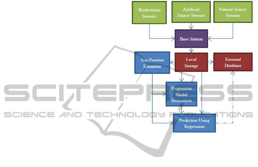
3.2 System Architecture
The wireless sensor network was programmed in
TinyOS, an open-source platform developed at UC
Berkeley (Levis et al., 2005). A flowchart for the
software structure can be seen in Figure 1. The
motes, each with their own unique ID’s,
communicate data packages to a base station mote
which forwards the data via a serial connection to a
computer which saves the data locally and forwards
it to an online database following a Simple
Measurement and Actuation Protocol (sMAP).
sMAP is being developed by UC Berkeley as a
single web based platform for accessing large
volumes of data from all possible sensor points from
a multitude of disparate and distributed data sources
such as building management systems of large
commercial buildings, ad-hoc sensor networks, grid
data from Intelligrid, building models from
GreenXML source, pricing data from OpenADR,
(Automated Demand Response) and monitoring by
Smart Energy Profile applications (Dawson-
Haggerty, 2011); (Dawson-Haggerty et al., 2012).
A Java-based program performs several tasks.
First, the data are parsed to fill in any gap caused by
lost packages. Second, the data from each mote are
then divided, depending on the angle of the sun at
each time step, which is computed using the
Astronomer Almanac’s sun positioning algorithm
(Michalsky, 1988). A daylight model is generated
through linear regression on a data set with no
artificial light (such as data taken over the weekend)
to create a piecewise linear function for each
workstation, divided by angle of inclination of the
sun. A linear function is estimated for every 1.0° sun
elevation. The daylight model is then extended to
create a full model using data sets with artificial
light.
Figure 1: Software flowchart.
3.3 Deployment
Sensors were deployed at the Sustainability Base at
NASA Ames Research Center across two cubicles in
an open-plan office space. Seven sensors were
deployed at or near the workplane and two sensors
were placed on the walls near the windows. Sensors
1, 2 and 3 were located at incremental distances
from the window mote 8, covering the workplane
across the entire cubicle and sensors 5, 6 and 7 were
replicated in the adjoining cubicle with 9 being the
window mote. Sensor 4 was located on top of a low
height partition between the two cubicles. The
sensors collected data for several weeks, reporting
the data to a local server, which forwarded the data
to an online data visualization page for remote
access.
Power level data from the controllable luminaries
were collected from the luminary system data logs
after the tests, to avoid invasive procedures that may
void the luminary warranty. The light level data
were then input into the inverse model generation
package.
Daylight model training data were sampled every
five minutes from May 25 – May 27, 2012, a
weekend during which no luminaries were turned
SENSORNETS2013-2ndInternationalConferenceonSensorNetworks
216
on. The full model training data were sampled from
May 25 – June 5, 2012.
4 RESULTS
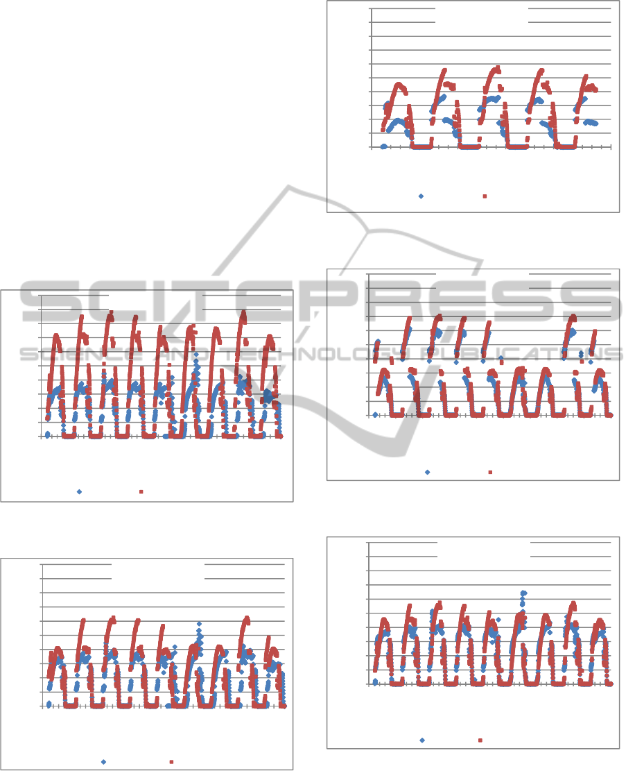
The full model was tested from June 11 – June 20,
2012. During this time, the building was occupied
and experiencing normal operations. The graphs for
the predicted values and measured sensor readings
are shown for workstations 1 – 7 in Figures 2 – 8,
respectively. The standard deviation of the residuals
and the root-mean-square error for each workstation
can be found in Table 1.
From Figures 2-8, it is apparent that our model’s
prediction errors are consistently higher for
workstations 1-3 compared to workstations 4-7.
Figure 2: Measured and predicted values of illuminance
for Workstation 1.
Figure 3: Measured and predicted values of illuminance
for Workstation 2.
Figure 4: Measured and predicted values of illuminance
for Workstation 3.
Figure 5: Measured and predicted values of illuminance
for Workstation 4.
Figure 6: Measured and predicted values of illuminance
for Workstation 5.
0
100
200
300
400
500
600
700
800
900
1000
11-06-2012
12-06-2012
13-06-2012
14-06-2012
15-06-2012
16-06-2012
17-06-2012
18-06-2012
19-06-2012
20-06-2012
Illuminance (lux)
Workstation 1
Measured Predicted
0
100
200
300
400
500
600
700
800
900
1000
11-06-2012
12-06-2012
13-06-2012
14-06-2012
15-06-2012
16-06-2012
17-06-2012
18-06-2012
19-06-2012
20-06-2012
Illuminance (lux)
Workstation 2
Measured Predicted
0
100
200
300
400
500
600
700
800
900
1000
11-06-2012
12-06-2012
13-06-2012
14-06-2012
15-06-2012
16-06-2012
Illuminance (lux)
Workstation 3
Measured Predicted
0
100
200
300
400
500
600
700
800
900
1000
11-06-2012
12-06-2012
13-06-2012
14-06-2012
15-06-2012
16-06-2012
17-06-2012
18-06-2012
19-06-2012
20-06-2012
Illuminance (lux)
Workstation 4
Measured Predicted
0
100
200
300
400
500
600
700
800
900
1000
11-06-2012
12-06-2012
13-06-2012
14-06-2012
15-06-2012
16-06-2012
17-06-2012
18-06-2012
19-06-2012
20-06-2012
Illuminance (lux)
Workstation 5
Measured Predicted
InverseModelingusingaWirelessSensorNetwork(WSN)forPersonalizedDaylightHarvesting
217
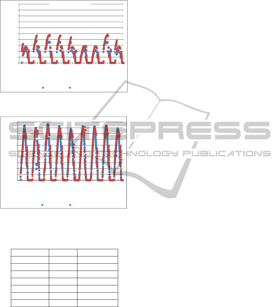
Figure 7: Measured and predicted values of illuminance
for Workstation 6.
Figure 8: Measured and predicted values of illuminance
for Workstation 7.
Table 1: Standard deviation of residuals and root mean-
square error for predicted values for workstations 1-7.
Workstation SD (lux) RMSE (lux)
1 204.32 257.76
2 108.65 142.715
3 211.61 213.06
4 86.90 91.44
5 58.78 61.56
6 55.66 62.17
7 92.51 101.93
5 DISCUSSION
The inverse model implemented from the dataset
obtained from our second test bed at NASA Ames
appears to predict the workstation light level with
higher accuracy than the previous tests on an
average. The root mean square error of the models
tended toward 100 lux or less on an average across
the monitored workstations except for a few of
workstations (1, 2 and 3), probably due to various
disturbances such as installed position and varying
traffic levels. The recommended lux level for
standard office work is 500 lux (IESNA, 2000) and,
assuming a logarithmic sensitivity of the human eye,
an average error of 100 lux is hardly perceivable.
While the standard deviation of the residuals for
some workstations is still very high, the majority of
the models exhibited standard deviations below half
of those reported in previous tests. Note that
accuracy and predictive capability of physically
based models of lighting, which use sophisticated
and computationally expensive ray tracing
algorithms, vary widely depending on the expertise
and the experience of the modellers, the average
being 20% (Ibarra and Reinhart, 2009).
The linear daylight regression model discretized
by solar tilt appears to be more accurate than single
linear regression models, with standard deviations of
residuals being up to 87.6% lower than those
reported in previous related work depending on the
sensor position (Guillemin, 2003).
5.1 Error Sources and Corrections
The possible major errors were expected to stem
from sensor accuracy and precision followed by the
complex nature of daylight spatial geometry like
distance from the windows, solar shading,
distribution of indoor reflective surface and
miscellaneous disturbances like occupant traffic,
change in sensor position and so on. The complex
nature of daylight is attributed to unpredictability of
weather parameters such as sudden cloud cover and
relationship of the building geometry to solar
geometry. Fluctuating weather patterns could affect
the correlation of illuminance values between the
motes at the workstations and those at the windows.
One solution to the first error would be to use
multiple motes and take advantage of data
redundancy, facilitated by temporary sensor platform
deployment for model identification (Wen, 2008).
Alternatively, an adaptive modelling algorithm
could be designed to appropriately deploy means of
data validation and fusion iteratively until a shared
performance goal is reached. For example, in our
study, a preliminary comparison of window sensor 8
readings with three on-site roof-mounted radiometer
data showed a good correlation between the two, but
not for sensor 9. Results of further comparison with
other reliable explanatory variables could eventually
be used to weigh the sensor 9 readings based on data
validity. We expect that sampling over a set of
0
100
200
300
400
500
600
700
800
900
1000
11-06-2012
12-06-2012
13-06-2012
14-06-2012
15-06-2012
16-06-2012
17-06-2012
18-06-2012
19-06-2012
20-06-2012
Illuminance (lux)
Workstation 6
Measured Predicted
0
100
200
300
400
500
600
700
800
900
1000
11-06-2012
12-06-2012
13-06-2012
14-06-2012
15-06-2012
16-06-2012
17-06-2012
18-06-2012
19-06-2012
20-06-2012
Illuminance (lux)
Workstation 7
Measured Predicted
SENSORNETS2013-2ndInternationalConferenceonSensorNetworks
218

cloudy and sunny days can indicate the possible
reasons for high standard deviations of the residuals
at workstations 3 and 4. This methodology calls for
interoperability with various information sources in
the building such as shading systems, BMS etc. – an
opportunity offered by sMAP. sMAP comes with
drivers written in Python for various data sources
found in standard building applications.
In places where both mean and standard
deviations of the errors are large, longer sampling
will allow disaggregating the effect of weather and
sun position from those of local disturbances on the
measured data at a given workstation. After sensor
placement, it was discovered that workstation 1 was
placed on a table that was raised and lowered by
nearly a foot and a half on a fairly regular basis,
likely contributing to the higher residuals and
standard deviation for that workstation. This
highlights a drawback to inverse modelling, in that if
the sensors are moved after initial placement, the
model becomes much less accurate. However,
occasional data exchange between motes and
comparison between the spatially distributed sensor
readings could again be used here to detect such
disturbances.
Sensor blockage due to occupant traffic could be
another potential source of error, which can be
addressed partly through sensor processing. Our
initial investigation of weekend and weekday data,
however, did not indicate any sharp change in data
pattern due to occupant presence.
Sun tilt cannot adequately explain the
relationship between solar geometry and building
geometry. The effect of 10° sun tilt might be
completely different in the morning and evening
depending on the building orientation. In our next
model we are trying to account for this factor by
dividing the data further by morning and afternoon.
From the above analysis, it is apparent that our
model should be capable of using several
explanatory variables when required, customized to
individual lighting scenarios with nodes that
exchange readings for time to time comparison.
Such a feature would be increasingly important for
the platform reuse model. Sandhu, Agogino A.M.,
and Agogino A.K. (2004) had proposed an Multi-
agent system (MAS) for distributed data processing
and Influence Diagram (Bayes’ net)-based decision
making in closed loop lighting control, the main goal
was to achieve flexibility of distributed computation.
We could formulate our case in a MAS framework,
in which individual workplane sensor may have its
own set of explanatory variables, while the common
goal of the supervisory algorithm would be to
minimize the average prediction error across the
spatially distributed agents.
6 FUTURE WORK
6.1 Extending Inverse Model for
Annual Energy Performance
Prediction
Some of the challenges of data driven-models are the
number of samples and perturbations required in
each of the model parameters to achieve a fairly
robust inverse model of a process. Developing a
calibrated physically-based model of the process can
address some of these challenges by obviating long
term data acquisition. We are creating and
calibrating a physically-based lighting model of the
monitored workspace at the Sustainability Base
using the RADIANCE lighting simulation software.
Outputs from the annual simulations of this model
will be used to extend and validate the reduced order
light model, which in turn will then predict the
energy and comfort performance of the control
algorithm.
6.2 Extending Inverse Model for Model
Predictive Control
The inverse light model of workstation lighting was
developed for the purpose of controlling individually
addressable luminaires. However, control of the sub-
systems of a complex system such as a building, or
even a cluster of buildings, must be more coupled as
engineers move beyond heuristic control approaches
and seek to incorporate predictive models of
occupancy, renewable energy availability and price
signals (Ma et al., 2012); (Liu and Henze, 2006),
accounting for interdependencies between energy
performance of these subsystems (Mukherjee et al.,
2010). This invites the challenge of controlling a
multi-input multi-output system where the response
time of the sub-systems varies from a few seconds to
several hours. Keeping in mind this challenge of
future smart building energy and comfort
management, we are using a modular approach to
augment our system identification platform. We are
extending the inverse lighting model for predictive
control of multiple smart shading systems, the
setpoints being instantaneously desired light level at
multiple workstations and desired zone temperature,
several time steps in the future.
InverseModelingusingaWirelessSensorNetwork(WSN)forPersonalizedDaylightHarvesting
219

7 CONCLUSIONS
Current market intelligent lighting control systems
seldom include a predictive light model within the
control loop and the implementations of these
systems have proven to be ineffective in the majority
of installations. The light sensors are mostly
overhead and tend to over-estimate the light level at
the workplane due to a different field of view than
the human eye at the workplane. Predictive models
of indoor lighting could also be integrated within the
framework of model predictive control of building
systems, an emerging strategy in the realm of smart
buildings on the smart grid.
As part of our research endeavour with the
Sustainability Base at the NASA Ames Research
Center we are developing a computationally
inexpensive predictive model of indoor lighting. To
this end we have deployed a low power wireless
sensor network at this test bed and developed a
piecewise linear regression model of workstation
illuminance, built on a month of data at seven
workstations, that was capable of predicting the light
levels within 36%-60% on average across the
workstations. We found that linear models
discretized by sun angles were able to explain and
predict the influence of daylight on workplane
illuminance better than previous related work that
considered only a single linear model as function of
vertical façade illuminance. However, in spite of a
low spatially averaged error we still noted higher
fluctuations of errors in the proximity of the
windows, in cubicles with higher occupant traffic or
when window motes receive more direct solar. In
order to address these error fluctuations we are
planning to develop an adaptive model that can
adjust the model coefficients based on system state.
Further using data from annual simulations of a
calibrated physically based model of the monitored
space, the current inverse model will be extended for
annual control algorithm generation and energy
performance evaluation. In addition we are
incorporating future daylight prediction capability
within the current model for better integration into a
model predictive control framework, including
systems of multiple response times.
ACKNOWLEDGEMENTS
This research has been supported by a grant from
National Aeronautics and Space Administration,
under the University Affiliated Research Centre
(URAC) award #NAS2-03144. The authors also
wish to thank and acknowledge the expertise and
valuable input from our NASA Ames colleagues
Adrian Agogino and Corey Ippolito, as well as intern
Edward Sullivan.
REFERENCES
American Society of Heating, Refrigerating, and Air-
Conditioning Engineers, Inc. (ASHRAE). (2010).
ASHRAE Standard Ventilation for Acceptable Air
Quality, Standard 62.1-2010. Atlanta: ASHRAE.
Ashe, M., Chwastyk, D., de Monasterio, C., Gupta, M.,
Pegors, M. (2012). 2010 U.S. Lighting Market
Characterization. Retrieved September 20, 2012, from
apps1.eere.energy.gov/buildings/publications/pdfs/ssl/
2010-lmc-final-jan-2012.pdf.
Brambley, M. R., Haves, P., McDonald, S. C., Torcellini,
P., Hansen, D., Holmberg, D. R., Roth, K. W. (2005).
Advanced Sensors and Controls for Building
Applications: Market Assessment and Potential R&D
Pathways. Oak Ridge: Pacific Northwest National
Laboratory.
California Energy Commission (CEC) and Itron Inc.
(2006). California Commercial End-Use Survey.
Retrieved November 14, 2012, from
http://www.energy.ca.gov/2006publications/CEC-400-
2006-005/CEC-400-2006-005.PDF.
California Public Utilities Commission. 2011. Average
Rate by Customer Class Years 2000-2011. Retrieved
November 14, 2012, from
http://www.cpuc.ca.gov/PUC/energy/Electric+Rates/E
NGRD/ratesNCharts_elect.htm.
Dawson-Haggerty, S. (2011). Introduction to sMAP.
Retrieved September 20, 2012 from
http://www.eecs.berkeley.edu/~stevedh/smap2/intro.ht
ml.
Dawson-Haggerty, S., Krioukov, A., Culler, D. (2012).
Experiences integrating building data with sMAP.
Retrieved September 20, 2012, from
http://www.eecs.berkeley.edu/Pubs/TechRpts/2012/EE
CS-2012-21.pdf.
Department of Energy, (2010). Buildings Energy Data
Book. Washington D. C.: Department of Energy.
Retrieved August 26, 2012, from
http://buildingsdatabook.eren.doe.gov/TableView.aspx
?table=3.1.4.
Deru et al. U.S. Department of Energy Commercial
Reference Building Models of the National Building
Stock. (2011). National Renewable Energy
Laboratories.
Guillemin, A., (2003). Using Genetic Algorithms to Take
into Account User Wishes in an Advanced Building
Control System. Ph.D.. École Polytechnique Fédérale
de Lausanne.
Hayashi, F., (2000). Econometrics. Princeton: Princeton
University Press.
Ibarra, D. I., Reinhart, C. F., (2009). Daylight Factor
simulation, How close do simulation beginners
SENSORNETS2013-2ndInternationalConferenceonSensorNetworks
220

“really” get?. In: Building Simulation, 11
th
International IBPSA Conference. Glasgow, Scotland.
27-30 July 2009.
Illuminating Engineering Society of North America
(IESNA). (2000). The Lighting Handbook, distributed
through the Illuminating Engineering Society of North
America, 9th edition.
Lee, E. S., Tavil, A., (2007). Energy and visual comfort
performance of electrochromic windows with
overhangs. Building and Environment, 42(6), pp.2439-
2449.
Levis, P., Madden, S., Polastre, J., Szewczyk, R., Woo, A.,
Gay, D., Hill, J., Welsh, M., Brewer, E., Culler, D.,
(2005). Tinyos: An operating system for sensor
networks. Ambient Intelligence, W. Weber, J. M.
Rabaey, and E. Aarts, (Ed.). New York: Springer
Berlin Heidelberg, 2005, 115-148.
Lindelhöf, D., (2007). Bayesian Optimization of Visual
Comfort. Ph.D. École Polytechnique Fédérale de
Lausanne.
Li, S. (2006). Wireless Sensor Actuator Network for Light
Monitoring and Control Application. In: Proceedings
of Consumer Communications and Networking
Conference, Las Vegas, NV, USA, January 8-10,
2006; 974-978.
Lin, Y., Megerian, S. (2005). Low Cost Distributed
Actuation in Large-scale Ad Hoc Sensor-actuator
Networks. In: Proceedings of 2005 International
Conference on Wireless Networks, Communications
and Mobile Computing, Maui, HI, USA, 2005; 975-
980.
Liu, S., and Henze, G., (2006). Experimental analysis of
simulated reinforcement learning control for active
and passive building thermal storage inventory, Part 1:
Theoretical foundation, Energy and Buildings, 38(2),
142–147.
Lu, J. and Whitehouse, K., (2012). SunCast: Fine-grained
Prediction of Natural Sunlight Levels for Improved
Daylight Harvesting. In: IPSN, 11
th
ACM Conference
on Information Processing in Sensor Networks.
Beijing, China. 16–20 April 2012.
Ma, Y., Kelman, A., Daly, A., Borrelli, F., (2012).
Predictive Control of Energy Efficient Buildings with
Thermal Storage: Modeling, Simulation and
Experiments, IEEE Control Systems Magazine, 44-64.
MEMSIC, Inc. (2012). TelosB_datasheet. Retrieved July
19, 2011, from
http://www.memsic.com/products/wireless-sensor-
networks/wireless-modules.html.
Michalsky J. J., (1988). The Astronomical Almanac’s
algorithm for approximate solar position (1950-2050).
Solar Energy, 40(3), 227-235.
Mukherjee, S., Birru, D., Cavalcanti, D., Das, S., Patel,
M., Shen, E., and Wen Y.-J., (2010). Closed loop
integrated lighting and daylighting control for low
energy buildings. Proceedings of the 2010 ACEEE
Summer Study on Energy Efficiency in Buildings,
Pacific Grove, CA, 2010.
Paulson, R. (2012). Personalized Illuminance Modeling
Using Inverse Modeling and Piecewise Linear
Regression. M.S. University of California, Berkeley.
Philips, (2011). Rapid-Prototyping Control
Implementation using the Building Controls Virtual
Test Bed. Philips Technical Report. Briarcliff Manor,
NY.
Rude, D. (2006). Why do daylight harvesting projects
succeed or fail? Construction Specifier, 59(9), 108.
Sandhu, J. S., Agogino, A. M., Agogino, A. K. (2004).
Wireless Sensor Networks for Commercial Lighting
Control: Decision Making with Multi-agent Systems.
In: Proceedings of Working Notes of the AAAI-04
Sensor Networks Workshop, San Jose, CA, USA, July
26, 2004; 88-92.
Singhvi, V., Krause, A., Guestrin, C., Garrett, J. H. Jr.,
Matthews, H. S. (2005). Intelligent Light Control
using Sensor Networks. In: Proceedings of SenSys'05,
San Diego, CA, USA, November 2-4, 2005; 218-229.
Tarantola, A., (2005). Inverse model theory and methods
for model parameter estimation. United States of
America: Society of Industrial and Applied
Mathematics.
Walton, M., Lee, E. S., Clear, R. D., Fernandes, L. L.,
Kiliccote, S., Piette, M. A., Rubinstein, F. M.,
Selkowitz, S. E., (2007). Daylighting the New York
Times Headquarters Building, Final Report:
Commissioning Daylighting Systems and Estimation
of Demand Response. Retrieved August 26, 2012,
from windows.lbl.gov/comm_perf/pdf/daylighting-
nyt-final-III.pdf.
Wen, Y.-J. (2008). Wireless Sensor and Actuator
Networks for Lighting Energy Efficiency and User
Satisfaction. Ph.D. University of California, Berkeley.
Wen, Y.-J., Agogino, A. M., (2011a). Control of Wireless-
Networked Lighting in an Open-plan Office. Journal
of Lighting Research and Technology, 43(2), 235-248.
Wen, Y.-J., Agogino, A. M., (2011b). Personalized
Dynamic Design of Networked Lighting for Energy-
Efficiency in Open-Plan Offices. Energy and
Buildings, 43(8), 1919-1924.
Wen, Y.-J., Bartolomeo, D. D., and Rubinstein, F, (2011).
Co-simulation Based Building Controls
Implementation with Networked Sensors and
Actuators. In: BuildSys, 3rd ACM Workshop on
Embedded Sensing Systems for Energy-Efficiency In
Buildings. Seattle, WA, USA. 1 November 2011.
InverseModelingusingaWirelessSensorNetwork(WSN)forPersonalizedDaylightHarvesting
221
