
Vision based Environment Mapping by Network Connected
Multi-robotic System
M. Shuja Ahmed, Reza Saatchi and Fabio Caparrelli
Materials and Engineering Research Institute, Sheffield Hallam University, Sheffield, U.K.
Keywords:
Environment Mapping, Object Detection, Computer Vision.
Abstract:
The conventional environment mapping solutions are computationally very expensive and cannot effectively
be used in multi-robotic environment, where small size robots with limited memory and processing resources
are used. This study provides an environment mapping solution in which a group of small size robots extract
simple distance vector features from the on-board camera images. The robots share these features between
them using a wireless communication network setup in infrastructure mode. For mapping the distance vector
features on a global map and to show a collective map building operation, the robots needed their accurate
location and heading information. The robots location and heading information is computed using two ceiling
mounted cameras, which collective localises the robots. Experimental results show that the proposed method
provides the required environmental map which can facilitate the robot navigation operation in the environ-
ment. It was observed that, using the proposed approach, the near by object boundaries can be mapped with
higher accuracy comparatively the far lying objects.
1 INTRODUCTION
Environment mapping is a process in which a robot
sense its surrounding using onboard perception sen-
sors and tries to obtain a global map. The generated
global map essentially helps the robots to navigate au-
tonomously in the environment. Environment map-
ping is a challenging problem to address and in most
cases, the robots require human assistance if they are
exploring the place first time. The main difficulty in
environment mapping is that the robots cannot know
their locations without having an environment map
and at the same time, the robots cannot build the en-
vironment map without knowing their locations. In
environment mapping problem, in the beginning, the
robots go around the environment while localising
themselves, keeps on building a map of what they
sense in the environment and this way, when they re-
visit a place, from the already generated map they get
some awareness of their surrounding. Once the full
map is obtained, then the robots can perform the path
planning efficiently, for example to determine a path
to reach some specific location. Some researchers
have worked around this problem in which the robots
keep on localising themselves and at the same time,
they also build the environment map. This is called
Simultaneous localisation And Mapping (SLAM) in
robotics field. In (Shen et al., 2008), a vision based
SLAM is presented in which the SIFT (Scale Invari-
ant Feature Transform) feature points are extracted
between the images to determine the robots’ updated
position and hence, it is used to determine the robots’
location and to map its trajectory. The use of vi-
sion based solution on one hand provides the rich
surrounding awareness to the robots but at the same
time, it increases the computational time consider-
ably. This leaves most of the vision based solutions
limited to be implemented using high performance
robots only. The current trend in robotics is shifting to
multi-robot operations in which a group of robots try
to achieve a common goal collectively (SYMBRION,
2008)(REPLICATOR, 2008). In multi-robotics oper-
ations, the robots being used have simple design to
reduce the cost of overall system. So a single robot
unit usually have limited onboard memory and pro-
cessing resources. For a single robot implementation,
researchers have used many different sensors such as
laser range finders, infrared sensors, sonar and vision
sensors. But most of the research is focused on us-
ing laser range finders. In (Wolf and Hata, 2009)
an approach to outdoor mapping is addressed using
2D laser range finder. Similarly, in (Kwon and Lee,
1999) a stochastic approach is adopted to an envi-
ronment mapping using laser range finder. From the
49
Ahmed M., Saatchi R. and Caparrelli F..
Vision based Environment Mapping by Network Connected Multi-robotic System.
DOI: 10.5220/0004314600490054
In Proceedings of the 3rd International Conference on Pervasive Embedded Computing and Communication Systems (PECCS-2013), pages 49-54
ISBN: 978-989-8565-43-3
Copyright
c
2013 SCITEPRESS (Science and Technology Publications, Lda.)

approaches adopted by (Wolf and Hata, 2009)(Kwon
and Lee, 1999), it can be seen that due to the phys-
ical size, high power and processing requirement of
the laser range finders, they are used with large size
robots. Moreover, a single laser range finder can cost
from £800 to £3000 which makes it unsuitable to be
used in multi-robotic environment where the objec-
tive is also to keep the cost of each robot unit low. In
(Biber et al., 2004), the information from the laser
scanner is fused with the vision sensor to provide
a more accurate map of the environment. But this
further increases the computational demands of the
approach. In (Howard, 2004)(Latecki et al., 2007)
a multi-robot environment mapping problem is ad-
dressed. But the results are limited to simulations
only. In (Leon et al., 2009), a grid based mapping
solution using multiple robots is addressed, but it also
utilised high performance systems.
When using a group of small size robots, it is pre-
ferred to use simple and computationally less expen-
sive algorithms such that, the task can be achieved
with limited processing resources. In this research,
a distributed vision based multi-robot environment
mapping problem is addressed in which a group of
robots collectively try to obtain a common global map
of the environment using the visual clues they ob-
tain from their surrounding. The generated map is
intended to facilitate the multi-robot mission planning
as the environmental map together with the robots po-
sition on the map will be available. The problem ad-
dressed here is different from SLAM as in this case,
the robots are provided the localisation information
from the ceiling mounted camera system. The robots
can share information through a wireless communica-
tion medium. This medium is usually prone to noise
and act as a bottle neck for information distribution.
So in this research, it is aimed that the robot relies
on simple visual features from the images such that it
does not overload the network and at the same time,
it is sufficient to map the environment collectively.
These visual features are represented in the form of
a vector which are extracted by determining the dis-
tance to the neighbouring object using vision informa-
tion. Knowing the robot camera field of view, this dis-
tance vector feature can be used to map the environ-
ment if precise robot location and orientation are pro-
vided. In the following sections, the complete multi-
robot environment mapping approach is presented.
2 METHODOLOGY
To address the multi-robot environment mapping
problem, two Surveyor SRV1 robots equipped with
the vision sensor were used. The Surveyor robot
(Surveyor-Corporation, 2012) is shown in Figure 1a.
For obtaining the robot localisation information, a
ceiling cameras based robot localisation system was
used. This system comprises of two ceiling mounted
cameras and a server system. Using the visual infor-
mation from the two ceiling mounted cameras, this
system is responsible to determine the robots’ posi-
tions, track them and pass them to the robots. Each
robot creates an environmental map in its memory.
This map is also updated by all the other robots work-
ing in the environment. For this purpose, each robot
gets its location and orientation information from the
localisation system. Once a robot knows its location
and orientation (as explained in Section 2.2), then
in the direction of its heading, it utilizes the visual
clues it obtained from its vision sensor and deter-
mines the surrounding objects boundaries. The robot
uses these detected boundary information to update
its own map. Apart from updating its own map, the
robot also broadcasts this map update information to
the other members in the environment. On receiving
this map update information, each robot in the envi-
ronment also updates their map. This way, each robot
in the environment not only knows the other robot’s
positions but at the same time, it also keeps on main-
taining a common map which is built by the contribu-
tion of all the robots in the environment. Each robot
also passes the map update information to the server,
which is running the ceiling cameras based locali-
sation system. This way, the map building process
can be seen on the server side. As the robots being
used have limited on-board memory and processing
resources, so it was decided to use a very light weight
vision algorithm to solve this problem. This problem
was divided into two parts, that is Objects’ Boundary
Detection, Robot Localisation and Mapping. These
are explained in the following sections.
2.1 Objects’ Boundary Detection
To determine the objects’ boundaries, a segmentation
based algorithm was used. A similar approach was
used by (Ahmed et al., 2012b), where it was utilized
to develop an efficient vision based obstacle avoid-
ance algorithm. The vision based obstacle avoidance
algorithm, addressed by (Ahmed et al., 2012b), also
works in parallel to help the robot control algorithm
to avoid colliding with obstacles. If the vision based
obstacle avoidance algorithm gives the ground clear-
ance signal to the robot control algorithm, then map-
ping algorithm is called which requires surrounding
objects’ boundaries information. To explain the con-
cept of segmentation based object boundary detection
PECCS2013-InternationalConferenceonPervasiveandEmbeddedComputingandCommunicationSystems
50
algorithm, an example image in Figure 1b is consid-
ered. After performing the segmentation of this im-
age, the resultant image is shown in Figure 1c. To
determine the distance to near by obstacles or to de-
termine the boundaries of the obstacles in the field of
view, the region covering the middle bottom of the
segmented image was considered for further process-
ing. After processing this region, the distance to the
boundaries of the objects, in the robot field of view,
were determined in pixels. The boundary information
was obtained in the form of a distance vector feature.
This feature vector provided the distance (in pixels)
to all the objects in robot’s field of view and is shown
in the Red colour in Figure 1d.
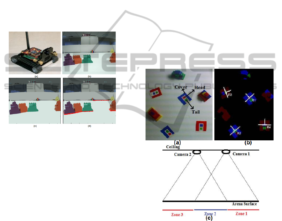
Figure 1: (a) Surveyor SRV1 robot. (b) Input image. (c)
Segmented image. (d) Distance vector feature.
2.2 Robot Localisation
Once the robots have computed the distance vector,
then to use this distance vector on the global map,
robots required their accurate location and heading
(orientation) information. For this purpose, a multi-
camera based robot localisation system, comprising
of two ceiling mounted cameras, was used. For robot
localisation, the system was programmed to recognise
coloured passive markers mounted on the top of the
robots. The passive markers recognition technique
is presented in detail in (Ahmed et al., 2012a). The
template used for the markers is shown in Figure 2a.
The localisation system identifies the Cover, Tail and
Head regions of the markers as identified in Figure
2a and determines the robot location and heading in-
formation as shown in Figure 2b (Four robots using
different colour markers are identified).
To provide robot localisation over the test arena,
the use of single camera was not sufficient as it does
not cover the entire arena. For this purpose, two ceil-
ing cameras were used. The entire arena was divided
into three zones and each ceiling camera was respon-
sible to localise the robots in different zones, as shown
in Figure 2c. Camera 1 covers zone 1 and 2, whereas,
camera 2 covers zone 2 and 3. As zone 2 is visi-
ble to both the ceiling cameras, so the robot local-
isation information in zone 2 is provided by fusing
the information from both the cameras. Both ceil-
ing cameras collectively localised the robots and pro-
vided this localisation information to the robots over
a wireless communication medium setup in the in-
frastructure mode. The localisation system provided
each individual robot the location information of all
the robots identified in the arena. This way, when
the robots generated the map using the distance vec-
tor information, they created a window around the de-
tected positions of other robots and avoided generat-
ing maps in those windowed regions. This helps to
avoid erroneous mapping of the boundaries detected
in the distance vector from the surfaces of the other
robots. This way, the boundaries detected from only
obstacles and arena walls are considered for mapping.
Figure 2: (a) Markers template. (b) Robots localisation and
heading. (c) Localisation system (Ahmed et al., 2012a).
2.3 Mapping
After computing the distance vector, the robots ob-
tained their locations and heading information pro-
vided by the ceiling cameras and mapped the distance
vector feature across their field of view. The robot
heading, obtained from the ceiling cameras, is iden-
tified by White coloured line in Figure 3a and the
robot field of view (i.e. 90 deg) is shown by the Red
and Yellow coloured lines. To map vector feature on
the global map, an equation is derived which trans-
VisionbasedEnvironmentMappingbyNetworkConnectedMulti-roboticSystem
51
lates the distance (in pixels) detected by the robot, to
the distance in image space of the ceiling cameras.
This is carried out because the robot is localised in
the image space of the ceiling cameras. To obtain this
equation, an object was placed at some distance from
the robot. Then the distances to the object, detected
by the robot and also by the ceiling camera, were
recorded. Ten experiments were performed while in-
creasing the object distance from the robot camera.
The data recorded are shown in Table 1.
Table 1: Scale factor: From robot to ceiling camera.
d
r
(Robot) d
c
(ceiling camera) Scale Factor(α)
(in pixels) (in pixels)
62 74 1.19
69 83 1.20
75 91 1.21
81 100 1.23
85 106 1.25
93 119 1.28
101 138 1.37
108 170 1.57
114 199 1.75
121 254 2.10
In Table 1, the first and the second columns show
the distance d
r
and d
c
detected by a robot and the ceil-
ing camera, respectively. The third column shows the
scale factor α between d
r
and d
c
. The scale factor is
obtained when d
c
is divided by d
r
and it is used to
translate the distance detected by the robot to the dis-
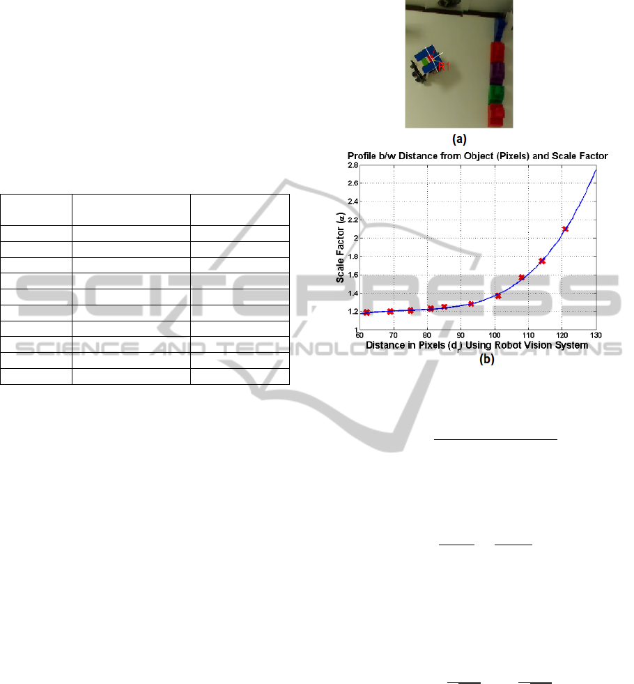
tance detected by the ceiling camera. In Figure 3b,
α is plotted against d
r
in Red colour and the fitting
equation (Eq 1) for this profile is obtained. The pro-
file generated using Eq 1 is also shown in the Blue
colour. From Figure 3b, it can be seen that the value
of scale factor varies depending upon the distance de-
tected by the robot. This shows that, objects detected
near the robot, will be mapped with higher accuracy
compared to far lying objects. Note that, as the vec-
tor of distance feature is generated, a vector of corre-
sponding values of α
i
also generated.
α
i
= 4.4e
−8
d
4
ri
−7e
−6
d
3
ri
+ 0.00011d
2
ri
+ 0.028d
ri
+ 0.0051
(1)
Where i = 1 → 320(Image width). When α
i
is
multiplied with d
ri
, then the corresponding values in
ceiling camera coordinates d
ci
is shown in Eq 2.
d
ci
= d
ri
α
i
(2)
From Figure 4a, d
ci
can also be described (Eq3)
in terms of the robot localisation (i.e. the coordi-
nates of robot position (x, y)) and the final coordi-
nates (x
mi
, y
mi
) where the object boundaries will be
Figure 3: (a) Robot field of view. (b) Fitting curve and
Profile b/w d
r
and α.
mapped.
d
ci
=
q
(x
mi
−x)
2
+ (y
mi
−y)
2
(3)
Similarly, the slope values s
i
(Eq4) for every d
ci
can
be computed using (x
ki
, y
ki
) (i.e. coordinates spanning
the robot field of view - see Figure 4a).
s
i
=
y
ki
−y
x
ki
−x
=
y
mi
−y
x
mi
−x
(4)
Now using the values of d
ci
along with the corre-
sponding slope values s
i
and the position coordinates
(i.e.(x, y)), the coordinates (x
mi
, y
mi
) can be computed
for mapping the object boundaries. The equation used
to compute x
mi
and y
mi
is shown in Eq5.
x
mi
y
mi
=
h
d
ci
√
1+s
2
i
+ x
s
i
d
ci
√
1+s
2
i
+ y
i
(5)
This way, once (x
mi
, y
mi
) are computed, the com-
plete distance vector feature is mapped to the ceiling
camera image space as shown in Figure 4b, where
the distance vector is plotted by the White coloured
line. The global map generated is also shown in Fig-
ure 4c. The image in Figure 4b is obtained from the
left ceiling camera. As two ceiling cameras are used,
the global map is obtained after using the information
from both cameras.
PECCS2013-InternationalConferenceonPervasiveandEmbeddedComputingandCommunicationSystems
52
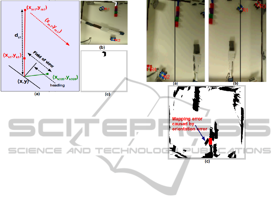
Figure 4: (a) Mapping process (b) Distance vector. (c) Map.
3 RESULTS
For experimentation, a test platform was designed
with obstacles placed in predefined forms and all the
robots were programmed to follow the boundaries in
the environment and map them. For robot localisa-
tion, the environment images provided by the left and
right ceiling cameras are shown in Figures 5a and 5b,
respectively. Four robots (labelled as R1, R2, R3 and
R4) were detected by the cameras. Robots R3 and R4
are not participating in the map building. They are
static, but as they are tagged with the passive mark-
ers, so they are detected as robots R3 and R4 by the
ceiling mounted cameras. Whereas, robots R1 and
R2 are working collectively to map the environment.
In these images, some blocks and boxes are placed
in the vertical direction to generate an environment.
The two robots R1 and R2 are expected to go around
in the environment and they will use the visual clues
from their vision sensor together with the information
from the ceiling cameras. This way they will map the
test arena boundary and walls made by the blocks.
The environment mapping process was a slow op-
eration because after every move, the robots needed
to wait so that the tracking system locks their current
position and provide them their location information.
This was done so that the robots are provided their
location and orientation information which precisely
represent their current position. This was important
as robots had to use this vision based location and
orientation information as the basis for mapping the
objects boundaries detected in the field of view of
their vision system. If this information corresponds
to the robot’s earlier position, then inaccuracies in the
map are expected. For example, a small error in the
orientation information can generate considerable er-
ror in the mapped boundaries. The two robots were
Figure 5: (a) Left ceiling camera image. (b) Right ceiling
camera image. (c) Map.
kept operative for 4 minutes and 21 seconds. After
the experiment finished, the generated map is shown
in Figure 5c. As mentioned before, a mapping error
caused by a small error in the detected robot orienta-
tion is also pointed out by the Blue coloured arrow in
Figure 5c. The actual location where this boundary
should be mapped is drawn in Red colour.
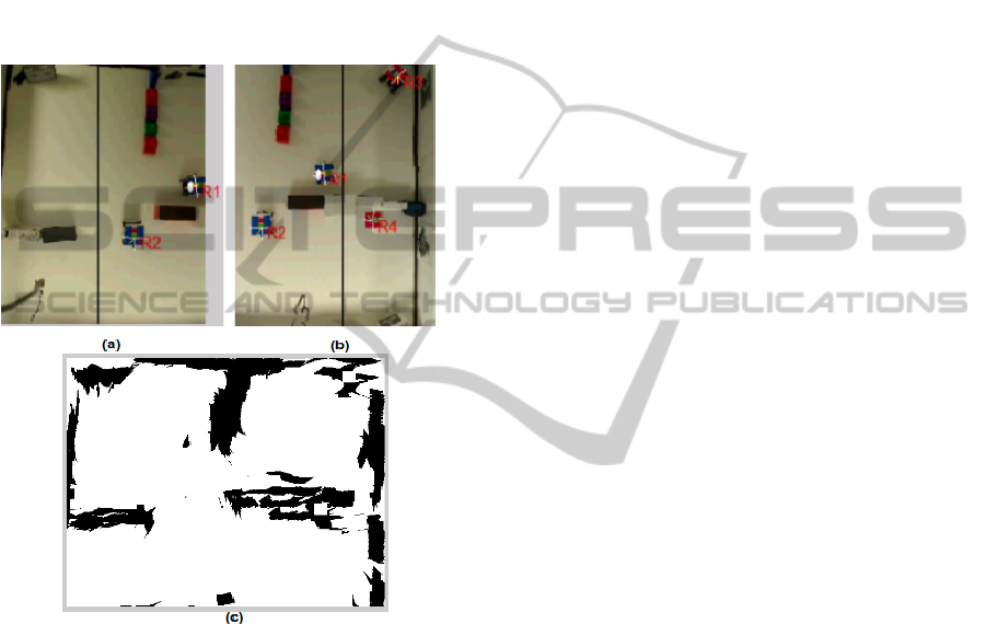
In another experiment, the environment was al-
tered by placing the objects in different order such
that they contribute to a different map. The place-
ment of objects for the generation of the new envi-
ronment is shown in Figures 6a and 6b. As the ob-
jective of this scenario was to demonstrate the collec-
tive vision based map building operation by a team
of robots rather than the efficient robotic control, so
the robot control algorithm performs simple vision
based boundary following operation. At the end of
the test, the robots have generated sufficient environ-
mental map as shown in Figure 6c.
In both the experiments 1 and 2, it was found that,
even after giving the location information of all the
robots to each individual robot, some of the bound-
aries resulted from the surfaces of static robots R3
and R4 were erroneously mapped (see Figure 5 & 6).
This happened because a square window region was
defined around the detected positions of the robots (as
discussed in Section 2.2) where as, the actual robots
used does not have a square shape (i.e., their length
VisionbasedEnvironmentMappingbyNetworkConnectedMulti-roboticSystem
53
and width is not same). As it was difficult to recognise
the pose of the robots (i.e., the robots detected in the
distance vector), so some of the boundaries detected
from their surfaces, got mapped erroneously. It was
also observed that, in both the experiments, some of
the regions remained un-mapped. This was expected
as the robots were not using any strategy to determine
which regions of the arena are mapped. To overcome
this, a path planning strategy can be used which in-
forms robots about the regions which needed to be
explored and mapped. This will also reduce the time
taken by the robots to map the environment.
Figure 6: (a) Left ceiling camera image. (b) Right ceiling
camera image. (c) Map.
4 CONCLUSIONS
We have proposed a method in which a simple vi-
sion based distance feature vector is computed and is
shared between the small size robots to generate en-
vironment map collectively. The accurate generation
of the map also depends on the precise robot location
and orientation information which is provided by the
ceiling mounted cameras. However, the use of simple
distance vector features not only facilitates the multi-
robot map building process, but it also does not over-
load the communication network between the robots.
The generated map can facilitate the robots to navi-
gate and solve the mission planning task in which the
detail environmental map is required.
ACKNOWLEDGEMENTS
Funded by EU-FP7 research project REPLICATOR.
REFERENCES
Ahmed, M., Saatchi, R., and Caparrelli, F. (2012a). Vision
based object recognition and localisation by a wire-
less connected distributed robotic systems. In Elec-
tronic Letters on Computer Vision and Image Analy-
sis, Vol.11, No.1, Pages 54-67.
Ahmed, M., Saatchi, R., and Caparrelli, F. (2012b). Vision
based obstacle avoidance and odometery for swarms
of small size robots. In Proceedings of 2nd Interna-
tional Conference on Pervasive and Embedded Com-
puting and Communication Systems, Pages 115-122.
Biber, P., Andreasson, H., Duckett, T., and Schilling, A.
(2004). 3d modeling of indoor environments by a mo-
bile robot with a laser scanner and panoramic camera.
In IEEE/RSJ International Conference on Intelligent
Robots and Systems (IROS). Vol.4, Pages 3430-3435.
Howard, A. (2004). Multi-robot mapping using manifold
representations. In IEEE International Conference on
Robotics and Automation(ICRA), Vol.4, Pages 4198-
4203.
Kwon, Y. and Lee, J. (1999). A stochastic map building
method for mobile robot using 2-d laser range finder.
In Journal of Autonomous Robots, Vol.7 No.2, Pages
187-200.
Latecki, L., Lakaemper, R., and Adluru, N. (2007). Multi
robot mapping using force field simulation. In Journal
of Field Robotics, Vol.24, Pages 747-762.
Leon, A., Barea, R., Bergasa, L., Lopez, E., Ocana, E.,
and Schleicher, D. (2009). Multi-robot slam and map
merging. In Journal of Phyical Agents, Vol.3, Pages
171-176.
REPLICATOR (2008). Robotic evolutionary self-
programming and self-assembling organisms. In
EU-FP7 Research Project REPLICATOR. URL:
http://symbrion.org/.
Shen, Y., Liu, J., and Xin, D. (2008). Environment map
building and localization for robot navigation based
on image sequences. In Journal of Zhejiang Univer-
sity ScienceA, Vol.9, No.4, Pages 489-499.
Surveyor-Corporation (2012). Surveyor srv-1 open source
mobile robot. In www.surveyor.com/.
SYMBRION (2008). Symbiotic evolutionary robot or-
ganisms. In European Communities 7th Framework
Programme Project No FP7-ICT-2007.8.2. URL:
http://symbrion.org/.
Wolf, D. and Hata, A. (2009). Outdoor mapping using mo-
bile robots and laser range finders. In Conference
of Electronics, Robotics and Automotive Mechanics,
Pages 209-214.
PECCS2013-InternationalConferenceonPervasiveandEmbeddedComputingandCommunicationSystems
54
