Making Sense to Modelers

Presenting UML Class Model Differences in Prose

Harald St

orrle

Department of Informatics and Mathematical Modeling, Technical University of Denmark,

Richard Petersens Plads, 2800 Lyngby, Denmark

Keywords:

Model based Development, Model Version Control, Model Difference Presentation.

Abstract:

Understanding the difference between two models, such as different versions of a design, can be difﬁcult.

It is a commonly held belief in the model differencing community that the best way of presenting a model

difference is by using graph or tree-based visualizations. We disagree and present an alternative approach

where sets of low-level model differences are abstracted into high-level model differences that lend themselves

to being presented textually. This format is informed by an explorative survey to elicit the change descriptions

modelers use themselves. Our approach is validated by a controlled experiment that tests three alternatives to

presenting model differences. Our ﬁndings support our claim that the approach presented here is superior to

EMF Compare.

1 INTRODUCTION

Motivation. In model based and model driven de-

velopment, code is increasingly being replaced by

models. Thus, model version control becomes a criti-

cal development activity for all but the smallest mod-

eling projects. (Kuhn et al., 2012) provide empir-

ical evidence to this claim. Consequently, version

control operators for models have attracted great at-

tention over the last years. For instance, there are

two ongoing workshop series on this issue, “Model

Evolution” (ME) and “Comparison and Versioning of

Software Models” (CVSM). The on-line bibliography

“Comparison and Versioning of Software Models”

(see (CVSM Bibliography, 2012)) records well over

400 publications in the area in the last 20 years, more

than 250 of which have been published in the last ﬁve

years. However, only less than ten out of these 250

publications consider the presentation of differences,

even though the best difference computation is little

use if the modeler cannot make sense of the change

report.

Apparently, it is a commonly held belief in the

model differencing community that the best way of

presenting a model difference is by graph or tree-

based visualizations, while text-based difference re-

ports are considered inferior. For instance, Ohst et al.

maintain that “the concept of [side-by-side presenta-

tion] works well with textual documents, [...but] does

not work well with graphical documents such as state

charts, class diagrams, etc.[...].” (cf. (Ohst et al.,

2003, p. 230)). Schipper at al. believe “that there is

a real need for a visual comparison” (cf. (Schipper

et al., 2009, p. 335)). Wenzel even claims that “The

textual presentation [of differences] [...] is very dif-

ﬁcult, or even impossible, to be read by human read-

ers” (cf. (Wenzel, 2008, p. 41)).

Approach. We disagree with this opinion. It is

certainly true that high-accuracy difference compu-

tations leads to very large numbers of low-level dif-

ferences, and simply dumping these to the user is

not very helpful: modelers are overwhelmed by

the amount of information they are confronted with.

There is, however, no reason, why we cannot try and

ﬁnd a more abstract textual difference representation

that is equally accurate but less detailed, and thus eas-

ier to understand for modelers.

Also, it is well known that conformance between

questions and answers increases task performance

and reduces cognitive load. We therefore propose

presenting model differences in the same terminology

and with the same aggregation size that modelers use

to describe changes in their models. This way, we

hypothesize, will modelers ﬁnd it more easy to un-

derstand model difference presented to them. In other

words: a model difference will make more sense to

a modeler if it is presented in the right terms. We ex-

Störrle H..

Making Sense to Modelers - Presenting UML Class Model Differences in Prose.

DOI: 10.5220/0004320900390048

In Proceedings of the 1st International Conference on Model-Driven Engineering and Software Development (MODELSWARD-2013), pages 39-48

ISBN: 978-989-8565-42-6

 2013 SCITEPRESS (Science and Technology Publications, Lda.)

plore this idea, formalize its notions, implement them,

and present empirical evidence comparing it to exist-

ing approaches.

Contribution. In this paper we propose an ap-

proach to compute model differences with maximum

accuracy, automatically derive high-level explana-

tions from them to reduce the level of detail, and

present these high-level differences in user-friendly

textual way. Our approach to version control of mod-

els looks at models as knowledge bases providing

an abstract view into some application domain. We

present a tool implementation of our approach and

brieﬂy evaluate its performance.

We report on two empirical studies discovering

the model change terminology and granularity used

by modelers, and exploring and comparing ways to

present model differences. We ﬁnd considerable ev-

idence in support of our hypothesis. The ideas re-

ported in this paper have evolved through a series of

papers (see (St

orrle, 2007b; St

orrle, 2007a; St

orrle,

2012)).

2 DIFFERENCE ALGORITHM

In the context of model comparison for version con-

trol, we typically want to compare two models that

are subsequent versions of the same model. Thus,

we can typically assume that (1) the two models have

been created using the same tool, and (2) they have a

large degree of overlap. This means, that both mod-

els use the same kind of internal identiﬁers for model

elements, and that most of the model elements have

the same identiﬁers in both versions. Thus, there is no

need to align models, and matching between their ele-

ments becomes trivial. These assumptions are clearly

not applicable in other, related areas, such as general

comparison of models, or model clone detection (see

e.g., (St

orrle, 2011a)). Note that EMF Compare (see

www.eclipse.org/emf/compare) has a wider focus and

includes an explicit matching phase before computing

model differences, although only identiﬁer and hash-

based matching seem to be currently available.

Mathematically speaking, we interpret a model as

a ﬁnite function from model element identiﬁers to

model element bodies, which are in turn ﬁnite func-

tions from slot names to values, which of course may

be (sets of) model element identiﬁers. We deﬁne the

following domains.

I Identiﬁers are globally unique elements.

S Slot names are identiﬁers that are unique in a given

model element, in meta-model based languages

like UML they correspond to meta-attributes.

V Slot values may be of arbitrary type, including ba-

sic and complex data types, and references to (sets

of) model elements.

B : P (S → V ) Model element bodies are maps from

slot names to slot values.

M : P (I → B) Models are maps from model ele-

ment identiﬁers to model element bodies.

We use the notation dom(f ) to denote the domain

of a function, and f ↓

to denote the restriction of

f to the sub-domain X ⊆ dom(f ). For example, if

f : A → B, then dom(f ) = A and f ↓

= {hx, f (x)i|x ∈

X,X ⊆ A}. The operator / denotes set difference, i.e.,

X/Y = {x |x ∈ X ∧x 6∈ Y }.

The domain deﬁnitions and notations introduced

above allow us to formulate the difference computa-

tion as basic set-operations. Let P and P

be two ver-

sions of a model, then the following deﬁnitions are

obvious.

Unchanged U = P ∩ P

Added A = P

↓

dom(P

)/dom(P)

Deleted D = P ↓

dom(P)/dom(P

)

Changed C = P

/(U ∪ A)

In order to compute the detailed changes of the

changed elements, similar deﬁnitions apply. For ev-

ery changed model element c ∈ C with identiﬁer i, we

deﬁne the following sets for the slots of C.

unchanged c

= P(i)∩ P

(i)

added c

= P

(i) ↓

dom(P

(i))

deleted c

= P(i) ↓

dom(P

(i))

changed c

= P

(i)/(c

∪ c

)

Clearly, all of these sets can be computed trivially

and efﬁciently. Observe that the result of applying

these operators are not necessarily consistent models.

For instance, if model P contains only a class A, and

model P

contains also a class B and an association

between A and B, then P

↓

dom(P

)/dom(P)

(the set of

added elements) contains class B and the association,

but not class A, that is, the association contains a slot

pointing to A, i.e., a dead link.

Algorithm 1 : Compute difference between two models

OLD and NEW .

function DIFF(OLD,NEW)

compute sets A, D, and C as deﬁned

for all c ∈ C compute c

, c

, and c

tag elements with their change type

return A ∪ D ∪

c∈C

∪ c

)

end function

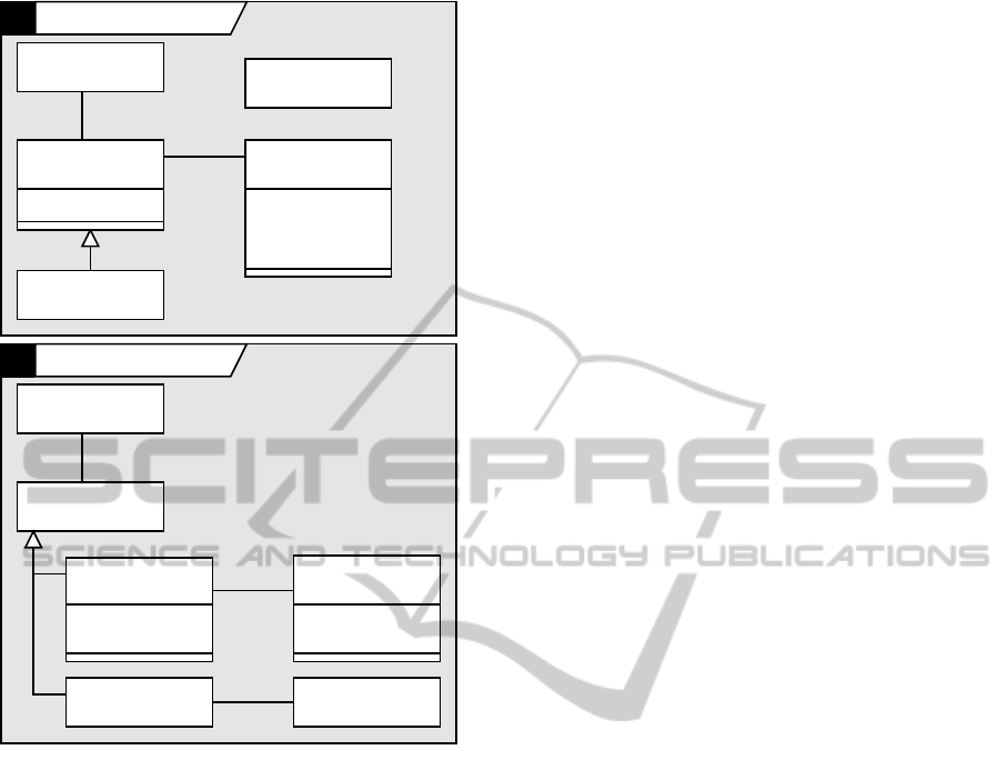
Consider the example in Fig. 1. It shows two sub-

sequent versions of a class model in the insurance do-

main. Obviously, this is only a small toy example with

a modest number of straightforward changes, ﬁnding

MODELSWARD2013-InternationalConferenceonModel-DrivenEngineeringandSoftwareDevelopment

CD Insurance Entities v.1

CD Insurance Entities v.2

PersonProduct

gender: Char

last change: Date

1..*

Supplier

LifePlan

validThru: Date

Person

Product

gender: String

Insurance

LifePlan

MedicalPlan

validThru: Date

signed: Date

Company

1..*

Date

renamed

moved

added

deleted

added

deleted

added

changed

added

moved

Figure 1: Running example for versioning models: orig-

inal version (top); and subsequent version (bottom), with

changes annotated in red.

all of them can be difﬁcult. But even a complete and

explicit list of the changes may be difﬁcult to read

if the number of changes grows too large. Even in

the small example from Fig. 1, there are 36 changes

between the two models, making this change report

difﬁcult to understand.

However, we have observed patterns in these low-

level change reports: usually, groups of changes oc-

cur together as the effect of a single modeling action.

Reconstructing these high-level changes from the low

level observations will improve the understanding of

model changes. This is the topic of the next section.

3 EXPLORING MODELERS’

DIFFERENCE PERCEPTION

In order to learn what concepts and abstractions mod-

elers ﬁnd helpful when talking and reasoning about

model differences, we explored modelers’ perception

of model differences through a qualitative study. We

created three pairs of sample UML class diagrams

that contained between 8 and 12 changes each. All

kinds and sizes of changes were covered at least

twice. We highlighted all changes by circling their

effect in the diagrams in red and numbering them ran-

domly. Fig. 2 (left) shows an example. Next we pre-

sented these model pairs to 4 graduate students and

asked them to describe the highlighted model changes

in their own words. We asked them to write down

their change descriptions, referring to the numbers

associated to the changes in the diagrams. We also

asked them to speak out loud what they were thinking

in the process and audio-recorded their utterances.

We found that there were three dimensions of vari-

ation in the ways study participants described model

differences. Firstly, there were variations in the gram-

mar and vocabulary, particularly the choice of verbs.

For instance, subjects might use “remove” instead of

“delete”, and “change” instead of “update”. Similarly,

subjects might use either present tense or past tense,

or even a mix of both when describing changes. Since

both of these variations appeared without any perceiv-

able pattern, we hypothesize that the variables gram-

mar and vocabulary are of little importance to model

change description. Mostly, subjects used the pas-

sive voice rather than the active voice or imperative.

For instance, the change marked 1 in Fig. 2 would be

described as “Class ’Date’ was deleted” rather than

“Delete Class ’Date’ ”. We attribute this to the fact

that it was not clear to the study participants who had

actually done the changes, so there was no obvious

grammatical subject to use in the change descriptions.

Secondly, some changes were described in a

generic way while others were described in a more

speciﬁc way. For instance, the change marked (2)

in Fig. 2 would always be described as a ’renaming’

rather than a change or update of the meta-attribute

’name’. In some cases, both types of change de-

scriptions could be observed. For instance, change

(3) would often be described as a decrease in ’Prod-

ucts’ associated to ’Persons’, but sometimes subjects

might also describe it as “change the multiplicity of

the association from 1..* to 1’. Similarly, changes to

the meta attribute ’isAbstract’ would usually be de-

scribed as ’making abstract’ or ’making concrete’ of

a class. There were yet other occasions, however,

where no speciﬁc description applied, and subjects

would use a variant of the generic description schema,

i.e., we would observe a change description like “The

type of feature ’gender’ was changed from ’Char’ to

’String’ ”. Generally speaking, most subjects pre-

ferred ’special case descriptions’ over the generic de-

scription pattern most of the time. Assuming that

MakingSensetoModelers-PresentingUMLClassModelDifferencesinProse

CD Insurance Entities v.1

PersonProduct

gender: Char

last change: Date

1..*

Supplier

LifePlan

validThru: Date

Date

You are looking at two versions

of a class model retrieved from

a version control systems. De-

cribe the changes made in the

second version!

(1) Class 'Date' was deleted.

(2) Class 'Supplier' was renamed to

'Insurance'.

(3) The number of 'Products' associ-

ated with a 'Person' was reduced

from 'one or more' to 'one'.

You are looking at two alterna-

ve versions of a class model.

Describe the diﬀerences be-

tween these two versions!

(1) V.1 has a class ‘Date’ while v.2 does

not.

(2) Class 'Supplier' in v.1 is called

'Insurance' in v.2.

(3) In v.2, a 'Person' is associated to

only one 'Product', while in v.1

there may be one or more.

Task Change Descripon

Figure 2: Exploration of change descriptions by modelers: model markup (left); change description as a function of task

description (right).

the subjects always tried to describe the changes in

the most accurate way they could, we concluded that

these changes were considered strictly different by the

subjects, and should be described in speciﬁc terms

rather than generic terms. However, there were some

changes that were described in rather different ways

by different subjects. For instance, changing general-

izations between classes, was described as ’let x in-

herit from y rather than z’ by one subject, while an-

other subject described it as ’replace z by y as gener-

alization of x’. We attribute this variation to different

degrees of UML-sophistication in the subjects, which

might mean that there should be different ways of de-

scribing the same change in different situations and to

different audiences.

Thirdly, we observed that the wording of the task

description had great inﬂuence on the change descrip-

tions produced by the subjects, as this description

would hint at an application scenario which lead sub-

jects to use different constructions matching the imag-

ined scenario. Consider the variants of task descrip-

tions and resulting change descriptions as shown in

Fig. 2 (right). These two scenarios describe models

as (A) subsequent or (B) alternative versions, i.e., as

dependent or independent of each other. In the former

case, descriptions typically used past tense and pas-

sive voice, using activity verbs like “add” or “delete”

to describes changes. In the latter case, change de-

scriptions typically contrasted two states using the

present tense of state-describing verbs, especially ’be’

or ’have’.

4 DIFF INTERPRETATION

Abstraction Rules. The overall idea is to provide

rules to explain sets of changes in a more abstract

way. For instance, if a class C is deleted, its transi-

tive parts and attached associations are also deleted.

So, computing the difference results in a large num-

ber of detail changes that might confuse the modeler.

This set of detail changes can often be replaced by a

single modeler-level explanation, e.g., something like

’deleted C and parts (cascading)’. Also, some changes

are more important than others, and some may be re-

ported summarily. For instance, changing the name

of a class is often more important than changing its

visibility. So we deﬁned the following rules for ab-

stracting low-level changes, based on observations

on change protocols of difference computations of a

set of modeling case studies (see (St

orrle, 2011a) for

more details on these case studies).

Rename. Replacing a change “update attribute

’name’ of class ’Supplier’ to ’Insurance’ ” into

“rename ’Supplier’ to ’Insurance’ obviously does

not reduce the number of changes, but makes it eas-

ier to understand the change.

Move. Moving an element from one container to an-

other changes the list of contained elements of both

containers, so a pair of low-level changes can be ac-

counted for with a single high-level change, and the

operation “move” is easier to make sense of than a

pair of addition and deletion, in particular if these

are not presented together.

Delete. Deleting an element also deletes its parts, re-

moves a link to it from the part-list of its con-

tainer, and any references from other elements to

it. Typically model elements have several parts,

which might again have parts so that deleting a sin-

gle element may cascade a number of times, and

a substantial number low-level changes can be ab-

stracted this way.

Add. Similarly, adding an element again also

changes the part-list of its container, often adds

MODELSWARD2013-InternationalConferenceonModel-DrivenEngineeringandSoftwareDevelopment

parts, and possibly references from other elements

to it. Furthermore, similar additions could be

grouped, such as when adding several properties

to a class: a single change can summarize such a

change set.

Associate/Dissociate. Adding or removing an asso-

ciation between some elements amounts to adding

or removing the element itself, its (transitive) parts

and properties, and references to these parts. For

instance, an association is a connection between

properties of the associated elements, and it is them

who own the properties rather than the association.

Re-associate. Exchanging one participant of an as-

sociation by another replaces a pair of overlapping

associate and dissociate-changes.

Tool Speciﬁc. Some changes refer to tool speciﬁc

elements such as extension elements, internal li-

braries and so on. These should be suppressed in

a high-level view.

Implementing these rules must satisfy two ma-

jor design goals. Firstly, the number of the reported

changes should be substantially reduced and their un-

derstandability increased (Goal 1: reduce number of

changes). Secondly, it should be easy to inspect a

high-level change and ﬁnd out what low-level changes

it actually accounts for, so that both the results and the

procedure are transparent (Goal 2: account for ab-

stractions). Thirdly, the rules should be independent

of each other such that it is easy to add or change them

(Goal 3: Independence).

Difference Abstraction Algorithm. In a ﬁrst at-

tempt, we tried to provide a set of explanation rules

that would consume the computed changes of a model

difference. This way, each high-level change could be

made to contain the low-level changes it accounts for

which would satisfy the design goals 1 (change reduc-

tion) and 2 (accountability). Such an algorithm works

ﬁne when considering only renaming, moving, and

additions/deletions of classes, properties, and similar

entities.

However, there are many cases where the same

low-level change can be explained by different ex-

planations. For instance, consider the following three

high-level changes possible to deduce from our above

rules.

• adding class ’Company’,

• associating class ’Company’ to class ’Medi-

calPlan’, and

• re-associating another class with ’Company’

All of these high-level changes would account for

the low-level changes “add anonymous property” and

“update ownedMember of ’Company’“. Of course,

creating a high-level change report should explain as

many low-level changes as possible, and so each rule

is “greedy”. This would imply that each rule must

have a great number of case distinctions that encode

deep knowledge about all other rules and what low-

level changes may or may not have already been ac-

counted for by another rule. Clearly, this contradicts

the third design goal (independence of rules). So, the

ﬁrst design of simply consuming low-level changes is

inadequate.

Instead we chose a different approach. If a high-

level explanation E is found to account for a set of

changes C = {c

,.. . ,c

}, then the elements of C are

marked as accounted for, and linked to their high-

level explanation E, while E is being added to the list

of computed changes. Clearly, this approach allows

to satisfy design goals 2 (accountability) and 3 (in-

dependence), but not 1 (reduce number of changes),

since the number of changes steadily increases. How-

ever, the number of changes not accounted for does

decrease, and so a slight variant of design goal 1 is in-

deed satisﬁed. This solution has the added beneﬁt that

there may now also be rules to abstract from previous

abstractions (e.g., rule “Re-associate”).

Since the number of low- and high-level changes

never reaches zero and we cannot know in advance

how far their number may be reduced, we use a ﬁxed-

point algorithm to implement this solution. In other

words, the rules are applied until the set of changes

does not change any further, which includes both the

overall size of the set and the number of accounted-

for changes. Conﬂicts between different explana-

tion rules need to be resolved by the programmer at

design-time; different orderings might result in dif-

ferent interpretations. The ﬁnal algorithm is shown

as Algorithm 2. Clearly, the algorithm terminates, if

there is at least one explanation for each change. We

achieve this by adding the default explanation, where

a change is explained by itself. This rule applies only

as a fall-back, i.e., if no other explanation applies ear-

lier.

As an added beneﬁt, this approach is indepen-

dent of the ordering in which rules for interpreting

low-level changes are applied. While the ordering of

model changes has no inﬂuence on the interpretation,

some sequences of operations are currently not de-

tected. For instance, deleting an element and creating

another element that is equal up to identity in another

place might be understood as a movement by a user,

but will not be recognized as such by the tool.

MakingSensetoModelers-PresentingUMLClassModelDifferencesinProse

Algorithm 2: Interpret difference D between two models

OLD and NEW .

function EXPLAIN(DIFF)

pick some d ∈ DIFF marked as ’fresh’

if there is an explanation E for change d then

ﬁnd largest D ⊆ DIFF explained by E

add E to DIFF

link D to E for tracing

mark E as ’fresh’ in DIFF

mark all D as ’stale’ in DIFF

end if

return DIFF

end function

function INTERPRET(DIFF)

mark all D ∈ DIFF as ’fresh’

DIFF

← DIFF

repeat

DIFF ← DIFF

DIFF

← explain(DIFF)

until DIFF = DIFF

remove all ’stale’ elements in DIFF

return DIFF

end function

5 IMPLEMENTATION

As in previous work on other model management op-

erations (see (St

orrle, 2011b; St

orrle, 2011a)), we

equate domain models with domain knowledge bases

and represent models as collections of Prolog facts.

Therefore, we have implemented our algorithm in

Prolog, too. There is a straightforward reversible

mapping between more conventional model formats

such as XMI and our Prolog representation.

Modelers can choose between different formats

for model difference, including low and high levels

of abstraction, and tabular or textual presentations.

Modelers are also offered statistics about the model

size, number of changes, and change rate.

Change Description Size. Using the running ex-

ample from Fig. 1, we may obtain difference reports

from EMF Compare, the low-level output from our

approach, and our high level output, presented in tab-

ular and textual format. In the remainder, we will

refer to these as treatments (1), (2), (3A) and (3B),

respectively.

Observe that the table and the prose text contain

identical information; they just present them in dif-

ferent formats. Clearly, EMF Compare uses by far

the most screen real estate to present changes, which

will be detrimental in maintaining an overview over

large differences. Also, the difference presentation of

EMF Compare is much more verbose without offer-

ing more information, while at the same time demand-

ing heavy interaction by the modeler inspecting the

differences when unfolding the difference tree. This

will likely increase the effort of the modeler in trying

to understand a model difference.

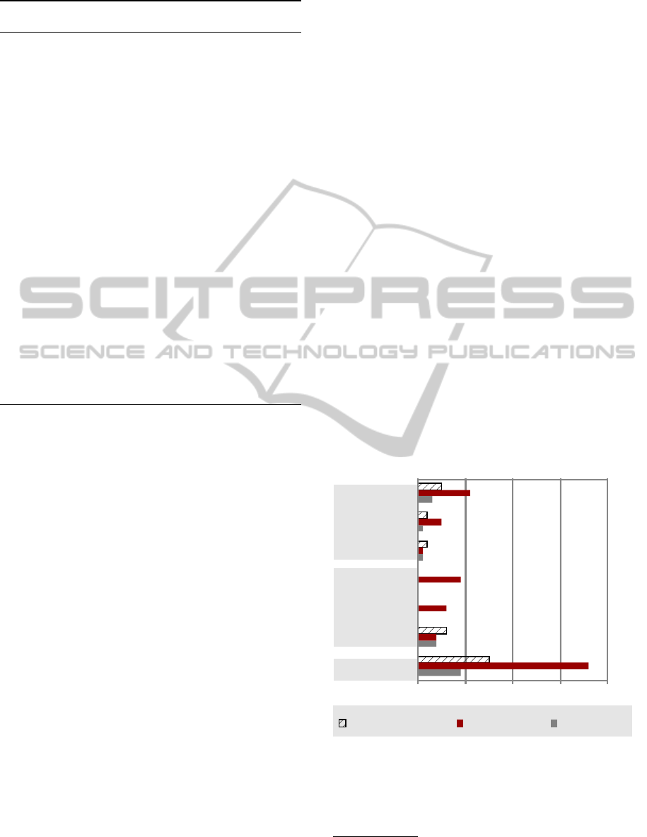
A quantitative comparison of the number of

changes is shown in Fig. 3. It is obvious that the

number of high-level changes is lower than the num-

ber of changes reported by EMF Compare, which

in turn is markedly smaller than the number of low-

level changes (36 vs. 15). Observe, however, that the

difference in numbers of changes reported by EMF

Compare and the low-level changes is almost en-

tirely explained by changes to the container attributes

(“ownedMember” et al.), and EMF Compare does not

report most of these changes.

Simply dropping this

type of information from the low-level change report

will result in almost identical numbers as compared

to EMF Compare. The number of high-level changes,

on the other hand, is notably smaller than the num-

ber of changes reported by EMF Compare (10 vs.

15). What is more important, however, is the way the

changes are presented in our approach, which we will

show to be much more understandable in Section 6.

10 20 30 40

Add

Delete

Move

Container

add

Container

del

other

Aributes Elements

Numbers of Changes by Type

Total

EMF Compare Low level High Level

Figure 3: Computational Performance.

Computational Performance. Contrary to com-

mon prejudice, using a high-level language like Pro-

log does not necessarily sacriﬁce run time for devel-

The exception being the order of the entries in one such

container attribute, which, conversely, our approach does

not consider.

MODELSWARD2013-InternationalConferenceonModel-DrivenEngineeringandSoftwareDevelopment

opment time. In fact, we have consistently observed

that our approach outperforms conventional Eclipse-

based tools, often by an order of magnitude or more.

In order to test this in the present setting, we have

timed a series of sample runs of our tool on a laptop

computer with an Intel Core i5-2520M, 2.5 GHz, 8GB

RAM under Windows 7. Fig. 4 summarizes our ﬁnd-

ings. It seems that both model size and change size

have an impact on execution time. The sample mod-

els range approximately from 1,000 to 2,000 model

elements, which makes them non-trivial, though not

extremely large. The response times are well below

a second, that is, our approach is practically viable.

A direct comparison to EMF Compare would require

instrumentation of the EMF Compare source code,

and is thus beyond our reach. Timing a user is in-

adequate, as EMF Compare requires interactions dur-

ing the differencing procedure. Discounting for these,

EMF Compare needs between 1 and 4 seconds for the

same models, i.e., it is considerably slower than our

approach.

100

200

300

400

500

600

700

800

3C 4C 2B 1A 4B

500

1000

1500

2000

2500

ChangesDuraon

Model Elements

(Base / Addions)

[ms]

[#]

Model Size vs. Diﬀerence Size

Figure 4: Relating model and difference size with run time:

the gray bars indicate the number of changes, the white

bars represent the sizes of two model versions by number

of model elements. The different case studies are plotted

left to right.

6 EVALUATION

Study Design, Materials, and Participants. We

validated our approach using a controlled experiment.

We prepared two pairs of diagrams with differences,

based on the models shown in Section 3. We removed

the change markup and created the difference descrip-

tions for each pair with EMF Compare and both our

own high level change descriptions, respectively. We

created a set of questionnaire sheets that display a pair

of models together with one of the difference presen-

tations and the instruction to check the difference de-

scription for correctness wrt. the diagrams shown. We

then combined two of these sheets into one question-

naire, permuting the sequence of the presentation for-

mats in different questionnaires.

We presented these questionnaires to 25 graduate

and undergraduate students; 17 of them returned a

questionnaire. All participants had an IT-related uni-

versity degree or were studying to obtain one. We

asked the subjects to validate the correctness of the

change presentations at their own pace. The tasks

were assigned randomly. A number of data points

were unusable because participants did not complete

all tasks or misunderstood tasks. Completion ranged

from 36% to 93% (average at 63%) depending on

treatments and measure.

Observations. We recorded the following three

variables:

• the number of errors (including both false nega-

tives and false positives);

• cognitive load (assessed subjectively through two

independent questions), recorded on a 5-point

Likert scale and later normalized to the interval

from 0 to 10;

• and the time used by the participants.

The observations are summarized in Table 1, a vi-

sualization is shown in Fig. 5. As the data clearly

show, subjects make two to three times as many errors

when using EMF Compare as compared to when us-

ing one of the other difference descriptions, although

they spend approx. 50% more time on the task. At the

same time, subjects report the highest subjective dif-

ﬁculty and lowest conﬁdence when using EMF Com-

pare. Interestingly, there is no large difference in both

objective measures (errors and time) for treatments

(3A) and (3B), while substantial differences in favor

of treatment (3B) can be observed in subjective as-

sessments.

Inferences. We have tested hypothesis of the form

“There are no differences wrt. x in modeler per-

formance for the three difference presentation for-

mats”, where x is number of errors, difﬁculty, conﬁ-

dence, and duration. As the distributions are strongly

skewed, we used the Wilcoxon test. Despite the small

number of replies in some categories, there are some

signiﬁcant results as shown in Table 2. We calculate

MakingSensetoModelers-PresentingUMLClassModelDifferencesinProse

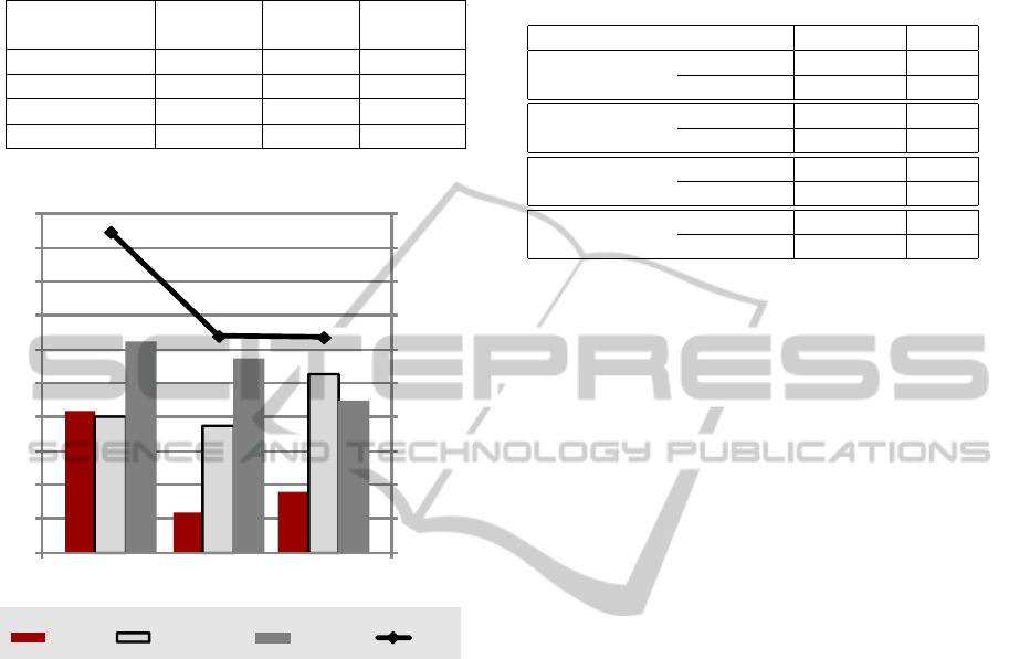
Table 1: Observations in our experiment: Conﬁdence and

Difﬁculty are normalized to a scale 0..10, time is in seconds;

Treatments are EMF Compare (1), Table (3A), and Prose

(3B).

TREATMENT (1) (3A) (3B)

µ(σ) µ(σ) µ(σ)

ERRORS 4.2 (2.0) 1.2 (0.7) 1.8 (1.6)

CONFIDENCE 4.0 (1.8) 3.8 (1.0) 5.3 (1.8)

DIFFICULTY 6.3 (1.3) 5.8 (1.5) 4.5 (1.5)

TIME 947 (348) 640 (56) 636 (390)

100

200

300

400

500

600

700

800

900

1000

EMF Compare

(1)

Table

(3A)

Prose

(3B)

Errors Conﬁdence

Diﬃculty

Time

Treatments ~ Measurements

Figure 5: Observations of the controlled experiment.

the effect size as Cohen’s d for the signiﬁcant results

and ﬁnd large effect sizes.

Overall, we conclude that treatment (1) – using

EMF Compare to represent model differences – is

signiﬁcantly inferior to both novel methods presented

in this paper. The data are not as clear when distin-

guishing between treatments (3A) and (3B), though.

Follow-up interviews revealed, that some subjects

were confused by the sequence in which the differ-

ences were presented. In particular, treatment (3A)

accidentally presented changes in a more intuitive

way than treatment (3B). As one subject put it: “The

table is better...I don’t have to jump around”. Simi-

larly, the prose presentation can be improved by pro-

viding more context to a given change. One partic-

ipant commented that “locating the elements [in the

diagram] takes too much time”. We conclude that

there is room for improvement that would likely im-

pact on the ﬁndings reported here.

Threats to Validity. There are several potential

threats to validity. We eliminated bias through the ex-

Table 2: Results of testing hypotheses “There is no differ-

ence in modeler performance for the change presentations

of EMF Compare vs. our approach” for different measure-

ments, with p-value of a one-tailed Wilcoxon test and Co-

hen’s d, showing large effect size.

MEASURE / TREATMENTS p d

1 vs. 3A 0.009 (**) 2.002

ERRORS

1 vs. 3B 0.016 (*) 0.755

1 vs. 3A 0.308

DIFFICULTY

1 vs. 3B 0.019 (*) 1.282

1 vs. 3A 0.567

CONFIDENCE

1 vs. 3B 0.943

1 vs. 3A 0.124

TIME

1 vs. 3B 0.102

perimenter by assigning the tasks randomly, provid-

ing only written instructions, and asked the subjects

to ﬁll in and return the questionnaires anonymously.

We eliminated bias through learning effects by pre-

senting all task permutations roughly the same num-

ber of times; any learning effects are canceled out this

way.

Bias through unrepresentative population sample

is controlled by a relatively large sample size (n = 25)

and by using three disjoint, relatively different pop-

ulations. All of the subjects are representative in

the sense that they are comparable to junior software

developers in the industry in terms of their exper-

tise. Observe that cultural bias can safely be excluded

since the participants came from more than 15 dif-

ferent (western) countries. Likewise, using class dia-

grams might be criticized as not representative for all

of UML. Indeed, collateral observations lead us to be-

lieve that different types of model might require very

different types of descriptions. However, class models

are by far the most commonly used of all UML dia-

grams, as Dobing and Parsons have repeatedly shown

(see e.g., (Dobing and Parsons, 2006)).

Another potential source of bias is the measure-

ment procedure, in particular wrt. cognitive load mea-

sures. We have taken two different measurements

that can be understood as aspects of cognitive load

(cf. (Paas et al., 2003)). Both of these measurements

show the same effect, though to varying degrees. Us-

ing subjective assessments rather than objective mea-

sures such as skin conductivity or pupillary dilatation

is justiﬁed by the high correlation between subjective

and objective assessments of cognitive load (cf. (Go-

pher and Braune, 1984)). Finally, the task formula-

tion could bias the outcome. However, the task was

presented in mostly visual form with no reference to

difference formats, with only very generic and brief

textual instructions.

MODELSWARD2013-InternationalConferenceonModel-DrivenEngineeringandSoftwareDevelopment

7 RELATED WORK

There are mainly two approaches to presenting model

differences, both of which are primarily visual. On

the one hand, model differences may be visualized

by color-highlighting different change states in the

diagrams used for presenting the model (see e.g.

(Girschick, 2006)). While initially quite appealing,

this approach has some severe limitations. First, us-

ing colors to differentiate element status is limited by

the number of colors humans effectively (i.e.: pre-

attentively) distinguish in a diagram. Long-standing

research in psychophysics informs us that this limit

is at ﬁve different colors (Bertin, 1981). Second, the

relatively wide-spread occurrence color vision deﬁ-

ciencies limits the effectiveness of this approach (up

to 10% of the western male popultion have partial or

total color blindness). Third, only those changes can

easily be represented by color highlighting that affect

elements presented in some diagram. Changes to the

model structure, say, or removal of hidden model ele-

ments (which is frequently the case for model clones)

have to be presented in different ways. Finally, even

those model changes that are presented in a diagram

might be difﬁcult to present when they affect more

than one diagram. For instance, consider the changes

done to a model as part of the rework assignment af-

ter a model review: this is likely to be spread out all

over the model and over several diagrams of different

types.

On the other hand, model differences may be vi-

sualized by side-by-side presentations of containment

trees of models, possibly enhanced by color coding

or connecting lines for movements (see e.g. the treat-

ment in EMF Compare). This way, some of the lim-

itations inherent in the ﬁrst approach are avoided: is-

sue relating to color vision are less important or can

be neglected altogether. Also, all changes can be dis-

played uniformly, whether the elements affected are

presented in a set of diagrams, a single diagram, or

no diagram at all. However, this approach does not

offer a satisfactory solution for large change sets: if

a model difference results in a large number of low

level changes, modelers can easily be overloaded by

the amount of information, resulting in confusion and

errors.

8 SUMMARY & RESULTS

In order to overcome problems with existing model

differencing approaches, we propose a new approach

to difference computation and presentation in this pa-

per. The difference computation and presentation we

propose here has been developed in a series of papers

(see (St

orrle, 2007b; St

orrle, 2007a; St

orrle, 2012)).

The current paper contributes numerous small im-

provements such as a better formalization of the do-

mains and algorithms, implementation, and perfor-

mance evaluation. The main contribution, however,

are the qualitative study to explore modelers’ under-

standing of changes, and the controlled experiment to

validate our approach.

These studies provide strong evidence to support

our hypothesis that a textual model difference presen-

tation can be as effective or even more effective than

the model difference presentation provided by EMF

Compare. Follow-up interviews reveal, that there is

further potential for improving the difference presen-

tations. We expect these to yield even clearer results

when testing.

REFERENCES

Bertin, J. (1981). Graphics and Graphic Information- Pro-

cessing. Verlag Walther de Gruyter.

CVSM Bibliography (2012). Bibliography on Compar-

ison and Versioning of Software Models. main-

tained by the SE group at the University of

Siegen, Germany, http://pi.informatik.uni-siegen.de/

CVSM/cvsm bibliography.html, last visited Septem-

ber 19th, 2012.

Dobing, B. and Parsons, J. (2006). How UML is used. Com.

ACM, 49(5):109–113.

Girschick, M. (2006). Difference detection and visual-

ization in UML class diagrams. Technical Report

TUD-CS-2006-5, TU Darmstadt.

Gopher, D. and Braune, R. (1984). On the psychophysics

of workload: Why bother with subjective measures?

Human Factors, 26(5):519–532.

Kuhn, A., Murphy, G. C., and Thompson, C. A. (2012).

An exploratory study of forces and frictions affect-

ing large-scale model-driven development. In France,

R. B., Kazmeier, J., Breu, R., and Atkinson, C., edi-

tors, Proc. 15th Intl. Conf. Model Driven Engineering

Languages and Systems (MODELS), pages 352–367.

Springer Verlag. LNCS 7590.

Ohst, D., Welle, M., and Kelter, U. (2003). Differences

between versions of UML diagrams. In Proc. 3rd Eur.

Software Engineering Conf. 2003 (ESEC’03), pages

227–236.

Paas, F., Tuovinen, J. E., Tabbers, H., and Van Gerven, P. W.

(2003). Cognitive Load Measurement as a Means to

Advance Cognitive Load Theory. Educational Psy-

chologist, 38(1):63–71.

Schipper, A., Fuhrmann, H., and Hanxleden, R. v. (2009).

Visual Comparison of Graphical Models. In Proc.

14th IEEE Intl. Conf. Engineering of Com plex Com-

puter Systems, pages 335–340. IEEE.

orrle, H. (2007a). A formal approach to the cross-

language version management of models. In Kuz-

MakingSensetoModelers-PresentingUMLClassModelDifferencesinProse

niarz, L., Staron, M., Syst

a, T., and Persson, M., edi-

tors, Proc. 5th Nordic Ws. Model Driven Engineering

(NW-MODE’07), pages 83–97. Blekkinge Tekniska

Hgskolan.

orrle, H. (2007b). An approach to cross-language

model versioning. In Kelter, U., editor, Proc.

Ws. Versionierung und Vergleich von UML Modellen

(VVUU’07). Gesellschaft f

ur Informatik. appeared in

Softwaretechnik-Trends 2(27)2007.

orrle, H. (2011a). Towards Clone Detection in UML Do-

main Models. J. Software and Systems Modeling. (in

print).

orrle, H. (2011b). VMQL: A Visual Language for Ad-

Hoc Model Querying. J. Visual Languages and Com-

puting, 22(1).

orrle, H. (2012). Making Sense of UML Class Model

Changes by Textual Difference Presentation. In

Tamzalit, D., Schtz, B., Sprinkle, J., and Pierantonio,

A., editors, Proc. Ws. Models and Evolution (ME),

pages 1–6. ACM DL.

Wenzel, S. (2008). Scalable visualization of model differ-

ences. In Proceedings of the 2008 international work-

shop on Comparison and versioning of software mod-

els, pages 41–46. ACM.

MODELSWARD2013-InternationalConferenceonModel-DrivenEngineeringandSoftwareDevelopment