
Incorporating Proofs in a Categorical Attributed Graph Transformation
System for Software Modelling and Verification
∗
Bertrand Boisvert, Louis F´eraud and Sergei Soloviev
IRIT, Universit´e Paul Sabatier, Toulouse, France
Keywords:
Model Transformation, Graph Transformation, Attribute Computation, Single Pushout.
Abstract:
This paper deals with model transformations based on attributed graphs transformation. Our approach is
based on the categorical approach called Single Pushout. The principal goal being to strengthen the attribute
computation part, we generalize our earlier approach based on the use of typed lambda-terms with inductive
types and recursion to represent attributes and computation functions. The generalized approach takes terms in
variable context as attributes and partial proofs as computation functions that permit to combine computation
with proof development and verification. The intended domains of application are the development of cerified
software models and semantics models for interactive proof development and verification.
1 INTRODUCTION
In Model Driven Engineering (abbreviated MDE),
models are mostly described using a graphical syntax
(UML, SDL, etc.). Models are composed of a struc-
tural part which can be represented as a graph and of
attributes which are informations attached to vertices
or edges of the graph. Thus, models can be formal-
ized as attributed graphs and model transformation as
attributed graph transformations. An attributed graph
transformation is composed of a rewrite of the struc-
tural part and of computations on its attributes.
When consideringgraph transformations,it can be
noticed that a lot of them deal onlywith structures and
not with attributes. For instance transforming UML
class diagrams to relational models or UML activity
diagrams to Petri nets require few attribute compu-
tations. In contrast, when dealing with formalisms
such as timed automata, complex Petri nets (predicate
Petri nets, Object Petri nets, colored Petri nets), in-
ternal program representation leads to sophisticated
attribute computations. In our previous and current
works we decided to focus on graph transformations
requiring complex computations. So we developped
a first approach based on a typed λ-calculus and now
we moved a step further considering inference rules
as a way to make attribute computations.
One of the challenges of attributed graph transfor-
mation systems concerns the implementation of at-
∗
Part of this research has been supported by the Climt
project, ANR-11-BS02-016-02
tribute computations. Most of the existing systems
based on category theory adopt the standard algebraic
approach where graphs are attributed using algebraic
data types represented by Σ-algebras (Ehrig et al.,
2006b), (Orejas, 2011). However, the computation
with algebraic data types does not permit to repre-
sent certain computations (like computation of recur-
sive functionsor term matching),and meets efficiency
problems when implemented.
In our earlier work, see (Rebout et al., 2011), (Re-
bout et al., 2008), (Tran et al., 2010) we suggested
to use inductive types and lambda terms in com-
bination with a modification of the double pushout
approach (Rozenberg, 1997) called DPoPb (“double
pushout-pullback” approach). As stated above, our
goal was to use a well developed approach to imple-
ment rewriting of the structural part of graphs and
to use the expressive power of λ-terms and induc-
tive types to describe and facilitate attribute compu-
tations. But the construction of the double pushout
imposed strong constraints on computation functions
mostly due to the usage of total maps and the obli-
gation to split all the computations into two parts.
That is why later we presented a new approach based
on single pushout and λ-terms as computation func-
tions (Boisvert et al., 2011a).
In this paper, we generalize this approach towards
models incorporating proofs. Instead of λ-terms in
the same fixed context we consider full typing judge-
ments of the form Γ ⊢ t : A where Γ is a context, t is
a term and A is a type. Instead of λ-terms as com-
62
Boisvert B., Féraud L. and Soloviev S..
Incorporating Proofs in a Categorical Attributed Graph Transformation System for Software Modelling and Verification.
DOI: 10.5220/0004321200620074
In Proceedings of the 1st International Conference on Model-Driven Engineering and Software Development (MODELSWARD-2013), pages 62-74
ISBN: 978-989-8565-42-6
Copyright
c
2013 SCITEPRESS (Science and Technology Publications, Lda.)

putation functions we take partial proofs in the corre-
sponding system of type theory. As a result, the scope
of the approach is considerably extended. It can be
used now not only to support attribute computations
in graph transformation systems but also in computer-
assisted verification and proof-development.
The next section of this paper introduces the main
approaches of graph rewriting based on category the-
ory, and particularly the single pushout approach on
which our approach is based. Afterwards we define
our category of attributed graphs, and then explain
how to apply a rewrite rule by the computation of
a weak pushout. Proofs are based on the ideas pre-
sented in (Boisvert et al., 2011a) but applied in more
general setting. In section 5 we present examples.
Section 6 contains an outline of future work. The pa-
per is completed by an appendix that contains a brief
description of the system of typed λ-calculus with in-
ductive types used for presentation and examples as
well as necessary notions of proof theory.
2 CATEGORICAL GRAPH
REWRITING
In graph rewriting systems based on category the-
ory, we usualy define a category whose objects are
graphs and morphisms are graph homomorphisms.
A transformation rule is composed of at least two
graphs called the left-hand side (usually noted L) and
right-hand side (usually noted R). The left-hand side
describes which subgraph a graph G must contain
in order that the transformation could be applied to
it, and the right-hand side describes how this part
will look like after the transformation. Morphisms
between left-hand side and right-hand side describe
which parts of graphs will be deleted, transformed or
added. To apply a rule to some subgraph of a larger
graph G, we need first to embed the left-hand side as
a subgraph of G. The embedding is represented by an
inclusion L
i
→ G. Cf Figure 1(a) and 1(b).
There are two principal categorical approaches to
graph rewriting: double pushout (abbreviated DPo,
concieved by H. Ehrig and his colleagues (Ehrig,
1978), (Rozenberg, 1997)) and single pushout (ab-
breviated SPo, mainly developped by L¨owe (L¨owe,
1993), (Rozenberg, 1997)). The main difference is
that in DPo morphisms are total maps andin SPo mor-
phisms are partial maps. This implies different forms
of rules.
In the DPo approach a rule is defined by 3 graphs
and 2 total morphisms: L
l
← K
r
→ R. The morphism l
indicates what vertices or edges should be erased (the
ones who are not in the image of l) and the morphism
r indicates what vertices or edges should be trans-
formed (those who are in K), and added (those who
are not in the image of r). The application of the rule
is done by a computation of a pushout-complement
(adding the arrows K
d
→ D and D
l
∗
→ G and then a
pushout (the arrows R
i
∗
→ H and D
r
∗
→ H). Cf Figure
1(a).
In the SPo approach, a rule is defined by one par-
tial morphim L
r
→ R. Vertices and edges not included
in the domain of r will be deleted, the ones in the do-
main of r will be transformed and those which are not
in the image of r will be added. The application of
the rule is done by the computation of one pushout
(adding the arrows G
r
∗
→ H and R
i
∗
→ H). Cf Figure
1(b)
L
i
K
l r
d
(PO1) (PO2)
R
i
∗
G D
l
∗
r
∗
H
(a) DPo approach
L
i
r
R
i
∗
(PO)
G
r
∗
H
(b) SPo approach
Figure 1: Classical categorical graph rewriting approaches.
Because not all pushout-complements necessarily
exist in the categories of graphs, there exist “applica-
tion conditions” in DPo approach. As a consequence,
rules that create dangling edges are forbidden in the
DPo approach while in SPo approach dangling edges
are removed when the rule is applied. If necessary, it
is possible to add application conditions in the SPo
approach as well. Thus the SPo approach is more
general than the DPo approach, but SPo approach re-
mained less developed due, in our opinion, mostly to
historical reasons and to the fact that computation of
pushout in categories of partial maps is more difficult
than in categories of total maps.
Both approachesmet many difficulties on the level
of attribute computations. Our experience with the
DPoPb approach, see (Rebout et al., 2008), (Rebout
et al., 2011), (Tran et al., 2010) and the use of λ-terms
for attributes was encouraging but the construction of
IncorporatingProofsinaCategoricalAttributedGraphTransformationSystemforSoftwareModellingandVerification
63

a double pushout still imposed some constraints due
to the use of total maps and the obligation to split
computation into two parts. The approach based on
single pushout construction with λ-terms as attributes
that we pursued afterwards (Boisvert et al., 2011a)
was more direct and natural, free of application condi-
tions and no specific constraints on the computational
level. It permitted to strengthen attribute computa-
tions and lighten the structure rewrite. At the same
time, while the relationship between λ-calculus and
proof theory is well known (one may mention famous
Curry-Howard isomorphism), the early version of our
system could not be used directly in proof develop-
ment and verification. In this paper, we generalize it
in this direction.
3 CATEGORY OF ATTRIBUTED
GRAPHS
To develop a categorical graph rewriting system we
must define a category (objects and morphisms) and
then explain how to apply a rule (in our case by the
computation of a pushout).
Let us recall that a pushout of two morphismsL
r
→
R, L
i
→ G is a couple of morphisms (G
r
′
→ H, R
i
′
→ H)
such that:
• i
′
◦ r = r
′
◦ i
• for every other couple of morphisms (R
h
→ H
′
,
G
g
→ H
′
) such that h ◦ r = g ◦ i it exists a unique
morphism c such that the diagram below com-
mutes:
L
i
r
R
i
′
h
G
g
r
′
H
c
H
′
As a consequence, the existence of pushout im-
plies the uniqueness of the object H up to isomor-
phism (cf. (Ehrig et al., 2006a), (L¨owe, 1993)). If we
have the two properties in the definition of pushout
but not the unicity of c, the construction is called a
weak pushout.
As in our previous work (Boisvert et al., 2011a),
the system T of λ-calculus is used to define attributes
and computation functions, but now we generalize
both the notion of an attribute and of a computation
function: instead of λ-terms in a fixed context, full
typing judgements Γ ⊢ M : A with arbitrary context Γ
and partial typing proofs are considered. The result-
ing category of attributed graphs will be denoted by
Gr
TP
. (For all notions that are not explained in the
main part of our paper please see Appendix.)
To have better idea of the power of T, let us recall
that it is a system of simply typed λ-calculus with sur-
jective pairing, terminal object and inductive types.
Type constructors include → for functional types, ×
for product(pairing) andInd for inductivetypes. Pair-
ing may be used to represent records, i.e., to “pack”
multiple attributes into one. The presenceof inductive
types permits to define all ordinary types of attributes,
like Bool, Nat, etc., as well as more complex types
like lists, binary trees, ω-trees, etc. Definition of in-
ductive types includes structural recursion over each
inductive type, this explains their particular interest in
modeling computations.
Below Θ is the set of all typing judgements of T.
Objects. Objects of Gr
TP
are attributed graphs.
An attributed graph is defined as 5-tuple G =<
V
G
,E
G
,sr
G
,tg
G
,att
G
>, wherethe structural part (first
4 items) consists of the set of vertices V
G
, the set of
edges E
G
and two functions source sr
G
: E
G
→ V
G
and
target tg : E
G
→ V
G
to connect edges to vertices. The
elements of the set V
G
∪ E
G
are called “elements of
the graph”. In this paper, we assume that V
G
∪ E
G
is fully ordered (lexicographically)
2
. The function
att
G
: V
G
∪ E
G
→ Θ associates exactly the judgement
Γ ⊢ M : A with each element of the graph.
To represent multiple attributes of a structural el-
ement, we use pairing to “pack” different data into
one λ-term. So each attribute can be seen as an n-
tuple containing all information attached to an ele-
ment. The n-tuple < M
1
,...,M
n
> is considered as an
abbreviation of the term < ... < M
1
,M
2
>,...,M
n
>.
Certain inductive type(s) can be reserved to rep-
resent labels in ordinary sense. E.g., let F
n
=
Ind(α){c
1
: α|...|c
n
: α} be a finite type. In T, we
have typing judgements Γ ⊢ c
i
: F
n
in any context Γ. If
we want to use c
i
in combination with other attribute
M : A, we may use < M, c
i
> of type A × F
n
. The
“absence of attributes” is represented by 0 : ⊤.
Morphisms. Let G,H be two attributed graphs. A
morphism f : G → H is defined in three parts:
1. The “structural part” noted f
str
is a partial graph
homomorphism (Rozenberg,1997) from the stuc-
tural part of G to the structural part of H (cf. Fig.
2).For each v ∈V
H
∪E
H
, its pre-image (i.e. the set
of all its antecedents) is noted [v]
f
str
⊆ V
G
∪ E
G
.
2. The “attribute dependency relation” f
adr
is a rela-
2
In any case, it is close to ordinary practice when ver-
tices are represented by natural numbers.
MODELSWARD2013-InternationalConferenceonModel-DrivenEngineeringandSoftwareDevelopment
64

tion between the sets V
G
∪ E
G
and V
H
∪ E
H
. For
each v ∈ V
H
∪ E
H
, its pre-image is noted [v]
f
adr
⊆
V
G
∪ E
G
. Applying to its elements att
G
, all at-
tributes of graph G which are used to compute v
can be obtained.
3. The “computational part” f
cmp
(v) is represented
by a partial proof. The partial proofs f
cmp
(v) have
to be “matched” with the attributes of G and H in
the following sense.
Let v ∈ V
H
∪ E
H
. Let att(v) = Γ ⊢ M : A. Let
[v]
f
adr
= {u
1
,...,u
k
},u
1
< ... < u
k
(as before, we
use the ordering on elements of G) and
att(u
1
) = Γ
1
⊢ M
1
: A
1
,...,att(u
k
) = Γ
k
⊢ M
k
: A
k
.
The partial proof tree p = f
cmp
(v) should have
exactly k active leaves with labels that are equal
to the attributes Γ
1
⊢ M
1
: A
1
,...,Γ
k
⊢ M
k
: A
k
(in
the order defined by the order of the leaves of the
tree). The root of the tree should have a label that
is equal to the attribute att
H
(v). Parameter leaves
are not matched to anything. (See Fig. 2.)
Equality of Objects and Morphisms. For objects,
we use identity on structural part and βηι-equality of
judgements of T for attributes. For morphisms, f = g
requires the identity of f
str
and g
str
, f
adr
and g
adr
; for
computation functions, for all v the equality of f
cmp
and g
cmp
(v) w.r.t. βηι-equality is required (see defi-
nition 6.5 of the Appendix
3
).
Categorical Structure on Gr
TP
. The identity id
G
is
defined using identity graph homomorphism as f
str
,
identity relation as f
adr
and canonical identity par-
tial proofs as f
cmp
(v). The composition of morphisms
(only the level of partial proof trees is non-trivial) is
defined using composition of partial proof trees, defi-
nition 6.6 of the Appendix.
Theorem 3.1. Gr
TP
defined above is a category.
Proof. Composition is associative due to associativ-
ity of the composition of graph homomorphisms, and
associativity of the composition of relations. For par-
tial proofs composition is associative too because of
confluence and the fact that T is strongly normaliz-
able. Thus any evaluation strategy will terminate on a
same simply typed λ-term. It is easy to verify that for
every morphism f : G → H we have f ◦ Id
G
= f and
Id
H
◦ f = f.
Remarks. This notion of equality is discussed in
detail in (Boisvert et al., 2011a). Here we would like
to remark that there is no reason to impose equiva-
lence relation on partial proofs themselves since the
3
We may obtain other interesting categorical structures
with different kinds of equality of judgements and partial
proofs, for example syntactic (graphical) equality of judge-
ments.
system we describe is intended to study the properties
of deductions, models etc. represented by attributed
graphs. So it is more natural to impose an equivalence
relation on attributes and attributed graphs as needed.
4 RULE APPLICATION BY A
WEAK PUSHOUT
COMPUTATION
As in the SPo approach, in our approach each mor-
phism r : L → R defines a transformation rule. The
auxilliary notion of an embedding is necessary to in-
dicate a “redex” - the part of the host graph to which
the rule can be applied.
Injective Attributed Graph Morphism. Let f :G →
H be an attributed graph morphism. f is injective if:
1. f
str
is an injective partial graph homomorphism
(i.e. ∀v
1
,v
2
∈ V(G) ∪ E(G).( f
str
(v
1
) = f
str
(v
2
) ⇒
v
1
= v
2
));
2. f
adr
= f
str
;
3. for each v
′
∈ V(H) ∪ E(H):
• if [v
′
]
f
adr
is empty, then f
cmp
(v
′
) is the partial
proof tree (cf. appendix) that has one node with
the label att(v
′
). It is at the same time its root
and its only leaf, which is not active.
• if [v
′
]
f
adr
is not empty (thus [v
′
]
f
adr
is a single-
ton because f
adr
is injective) then f
cmp
(v
′
) is
canonical identity partial proof for the attribute
att(v
′
).
We shall call an embedding a total injective at-
tributed graph morphism.
Canonical Retraction of an Embedding. Let f :
G → H be an embedding. A retraction of f (or a left
inverse) is an attributed graph morphism f : H → G
such that f ◦ f = Id
G
.
With this definition, we have not necessarily f ◦
f = Id
H
, and f is not unique in general. That’s why
we give a canonical construction to obtain a retraction
of f. This construction is defined by:
1. for every v
′
∈ V(H)∪E(H) if [v
′
]
f
str
is empty, i.e.,
v
′
does not belong to the image of f
str
, then v
′
does not belong to the domain of f
str
(v
′
); if [v
′
]
f
str
is not empty then [v
′
]
f
str
= {v} for some v because
of injectivity and we pose f
str
(v
′
) = v. Notice that
[v]
f
str
= {v
′
} by this definition.
2. f
adr
= f
str
3. for each v ∈ V(G) ∪ E(G) f
cmp
(v) is canonical
identity partial proof for the attribute att(v).
IncorporatingProofsinaCategoricalAttributedGraphTransformationSystemforSoftwareModellingandVerification
65
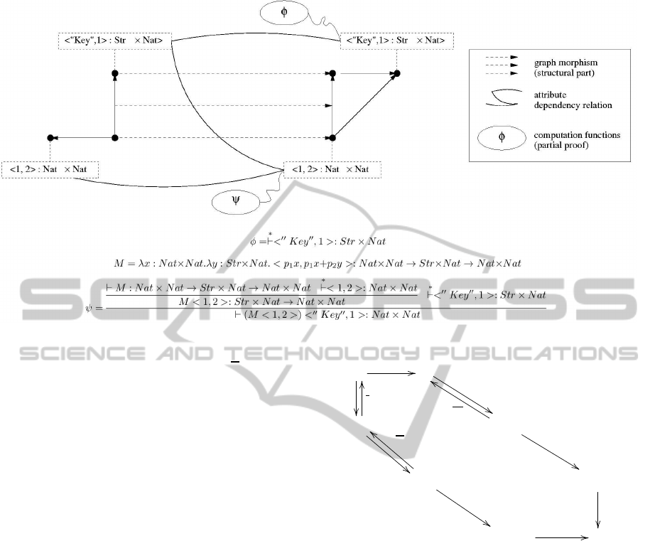
Figure 2: Attibuted graph morphism.
With this definition, it is easy to see that f ◦ f = Id
G
.
Construction of a Weak Pushout. The construction
of a (weak) pushout in case of application of a rule
is inspired by the paper by L¨owe and others (Rozen-
berg, 1997), but there will be differences due to our
definition of attributed graphs and graph morphisms.
The “starting point” is the pair of morphisms (L
r
→
R, L
i
→ G) where i is an embedding as definded above.
We want to compute the weak pushout (R
i
′
→ H, G
r
′
→
H) of this pair.
The first step to define a pushout would be to
take the coproduct G + R of G and R (coproduct be-
ing here just the disjoint union). Next step would be
to factorize it by certain equivalence relation (creat-
ing (G+ R)
′
which contains equivalence classes), and
then to complete the construction using composition
with certain morphism p from factor object to pushout
object H.
We shall define each of the morphisms r
′
and i
′
as
a composition of three morphisms (Cf. figure 3) in
order to have
r
′
= G
j
′
→ (G+ R)
f
′
→ (G+ R)
′
p
→ H
and
i
′
= R
j
′′
→ (G+ R)
f
′′
→ (G+ R)
′
p
→ H
The objects and morphisms in these diagrams are
defined in several steps.
• On the level of structure G+ R is disjoint union of
the graphs G and R;
L
i
r
R
j
′′
G
i
j
′
G+ R
f
′′
j
′′
G+ R
f
′
j
′
(G+ R)
′
p
(G+ R)
′
p
H
Figure 3: Construction of weak pushout.
• on the level of attributes each element of G and R
in G+ R has the same attribute as in G and R;
• j
′
and j
′′
are inclusions respectively of G and R
into G + R, thus they are total injective attributed
graph morphisms.
To continue, we define first the equivalence rela-
tion ∼
1
on the elements of the graph structure G+ R.
• let’s put a ∼
1
b for a,b ∈ G + R if ∃x ∈
L.( j
′
(i(x)) = a∧ j
′′
(r(x)) = b)
• then the relation ∼ is defined as reflexive, sym-
metric and transitive closure of ∼
1
.
• notice that the elements of G+R which are not the
images of elements of G−i(dom(r)) form equiva-
lence classes consisting of single element (itself).
The elements of (G + R)
′
are defined as equiva-
lence classes of elementsof G+R. It is easily checked
MODELSWARD2013-InternationalConferenceonModel-DrivenEngineeringandSoftwareDevelopment
66

that this definition is consistent with the incidence re-
lation and the map sending each element of G + R
to its equivalence class is a (total) graph homomor-
phism. This map will be structural part of f
′
and f
′′
.
Moreover, each equivalence class with respect to
∼ containingan image of an elementof R may be seen
as a “span”, consisting of the image of this element
of R under j
′′
and the images of its antecedent via
r under j
′
◦ i. In particular, each equivalence class
contains exactly one image of an element of R. As a
consequence, the composition f
′′
str
◦ j
′′
str
is injective.
It permits also to define the attribute part of (G+
R)
′
. Each equivalence class that contains an image
of an element of R has the same attribute as this ele-
ment has in R. Other equivalence classes (that have
the form { j
′
(y)},y ∈ G,y 6= i(x) for some x ∈ L) keep
the same attribute as in G.
The definitions of relational part and computation
functions of f
′
and f
′′
are different.
For f
′′
the relation f
′′
adr
connects the elements of R
with correspondingequivalence classes (it is bijective
on the R-part). There is no connections on the G-part.
The computation functions are identities.
Remark. The composition f
′′
◦ j
′′
is injective, in par-
ticular ( f
′′
◦ j
′′
)
str
is an injective total graph homo-
morphism,( f
′′
◦ j
′′
)
adr
= ( f
′′
◦ j
′′
)
str
and computation
functions are identities.
Now we may define f
′
as follows:
• ∀v ∈ img( j
′
◦ i):
f
′
= G + R
j
′
→ G
i
→ L
r
→ R
j
′′
→ G+ R
f
′′
→ (G+ R)
′
.
• for the elements of G−i(L), f
′
is like the identity.
As usual (cf. (Rozenberg,1997))H is defined now
as for coequalizer construction. Let L
0
= dom(r). In
our case H will be a subgraph of (G+ R)
′
. The inci-
dence relation in (G + R)
′
is inherited from R and G.
The elements on H (on the level of graph structure)
are:
1. all the equivalence classes of the form
{x
1
,...,x
k
,z} (x
1
,...,x
k
∈ j
′
(i(L
0
)),z ∈ j
′′
(r(L));
2. all the equivalence classes of the form {z}, z ∈
j
′′
(R− r(L));
3. all the equivalence classes of the form {x}, x ∈
j
′
(G − i(L)) that are not dangling edges (Rozen-
berg, 1997).
The attributes for the equivalence classes of the
first two types are inherited from R and for the third
from G.
The morphism p is defined as follows. Its struc-
tural part is identity on all elements of (G + R)
′
that
remain in H. We have also p
adr
= p
str
, and all com-
putation functions are identities.
Now i
′
, r
′
and H are defined such that i
′
◦ r = r
′
◦ i.
Let h : R → H
′
and g : G → H
′
be two other mor-
phisms such that h ◦ r = g ◦ i. As i
′
is injective, we
can use the canonical retraction i
′
and take for c h ◦ i
′
and for elements who are not in the domain of i
′
we
extend c in order to make it in accord with g. The
commutativity on the level of computation functions
follows from the definition of equality of attributed
graph morphisms (cf section 3). Thus the diagram
commutes but in general the unicity of c is not guar-
anteed, so we have a weak pushout.
This is summarised in the following theorem.
Theorem 4.1. Let L
r
→ R be an attributed graph
morphism and L
i
→ G be an embedding in Gr
TP
.
There exists weak pushout of L
r
→ R and L
i
→ G.
Moreover, it may be assumed that the morphism i
′
in
the (weak) pushout diagram is also an embedding.
Composite Rules. The proof of the theorem
above provides a canonical construction of the weak
pushout, in particular the vertical arrow i
′
is an em-
bedding like i. Such weak pushouts are sometimes
called specific weak pushouts because in the proof we
used the property that one of the two morphisms is an
embedding.
This construction of specific weak pushout per-
mits to compose the rules. Take two morphisms
L
r
→ R and R
r
′
→ R
′
. We have also their composition
L
r
′
◦r
−→ R
′
. The fact that i
′
in the specific weak pushout
above is also an embedding permits to construct the
second weak pushout representing an application of
the rule given by R
r
′
→ R
′
. It may be verified that the
construction of specific weak pushoutapplied directly
to r
′
◦ r gives the same graph H
′
after transformation.
Possible Generalizations: Schematic Morphisms
and Rule Schemas. The idea to use metavariables
in the definitions of graph transformation rules is sup-
ported by the practice of proof theory. Various ex-
amples are possible, e.g., one may define the disjoint
union of graphs using a rule schema (Boisvert et al.,
2011b). We shall use below only a restricted case of
rule schema based on the notion of schematic mor-
phism which we shall define precisely. For definitions
of partial proofs and schemas see Appendix, defin-
tions 6.4 and 6.8.
Definition 4.1. A schematic morphism is obtained
if we replace partial proofs in the definition of mor-
phism in Gr
TP
by partial proof schemas. An instance
of schematic morphism is any morphism in Gr
TP
ob-
tained by instantiation of metavariables. Let r : L → R
be a schematic morphism. The rule schema in Gr
TP
IncorporatingProofsinaCategoricalAttributedGraphTransformationSystemforSoftwareModellingandVerification
67

is the family of graph transformation rules defined by
all instances of r : L → R.
5 EXAMPLES
To illustrate our transformation approach we present
in this section two detailed examples that may be of
interest from the point of view of model transforma-
tions. The first one presents computationon attributes
representing infinite trees. This can not be done us-
ing Σ-algebras. Possible applications include trans-
formations of infinite models. The interest of dealing
with infinite models is now taken into consideration
(Combemale et al., 2012). A model can be infinite
according to the width or the depth of the graph. In
the example, we show how to deal with infinite width
trees. Another example concerns coercive subtyp-
ing, that has important uses in software modeling and
reuse (Soloviev and Luo, 2001).
Let us mention also some examples not devel-
oped in this paper that can be easily treated using
our approach: (i) graph cloning, cf. (Boisvert et al.,
2011b); (ii) generation and transformation of proofs
in deductive systems, cf. (Boisvert et al., 2012) (e.g.,
Kleene-style premutations of rules (Kleene, 1952));
(iii) information transfer between attributes and struc-
ture; (iv) transformations of UML diagrams to rela-
tional models; (v) term graph rewriting (cf. (Baren-
dregt et al., 1997)).
5.1 UML Diagram to Database
Relational Model
Our approach permits to manage classical graph
transformation problems like UML diagram to
database relational model transformation. This prob-
lem is described in (). In (Taentzer et al., 2005) the
transformation using the the DPo approach ... In our
approach it is possible to manage this classical prob-
lem. In this paper we present only an example of
rule because it would take several pages to present
them all. The figure 4 presents the rule “Class2Table”
(Taentzer et al., 2005). As we use typed λ-calculus, it
necessary to define the types used in this example:
• the type Type is defined as a finite type (see ap-
pendix 6) representing all “classes” of objects ma-
nipulated by the transformation:
Type = Ind(α){Class: α|Table : α|Column : α|...}
4
4
the constant Column and other constants are used in
other rules that are not described in this paper
• the type Connector is also defined as a finite type
representing all temporary nodes that permit to
connect elements of the class diagram to elements
of the relational database model (see (Taentzer
et al., 2005)):
Connector = Ind(α){C2T : α|A2C : α|A2F : α|...}
• the type Name is the type describing the Name of
the classes or tables. It is more or less like String.
• the type Bool is used as the value of the attribute
is persistent of a node of Type Class.
5
We do not describe only one rule of this problem
here because it would take several pages to write them
all, and there is no complex attribute computation in
these rules. Thus our approach has no advantage on
other approach to manage this example. It is possi-
ble to define all the other rules presented in (Taentzer
et al., 2005) in the same way.
5.2 Managing Infinity with Functional
Attributes
The use of λ-terms as attributes permits to manage
complex data structures that can represent infinity.
As an example, the type T
ω
which represents trees
with infinite branching
6
can be defined as follows:
T
ω
= Indα{0 : α,
S : α → α,
L : (Nat → α) → α}
Using the standard recursion operators on in-
ductive types (see appendix), we can define com-
plex ω-trees and computations on these infi-
nite tree structures. The figure 5 presents a
simple example of ω-tree defined by the term
L(Rec
Nat→T
ω
(0)(λx
Nat
λy
T
ω
.S(y))). It is also possible
to define computations that transform these terms.
It is possible to write a function that takes as ar-
gument an infinite tree, and give as results the trees
whith branches with pair numbers at every infinite
branching:
Rec
T
ω
→T
ω
(0)(λx
T
ω
.S)(λu.λv.(v◦ d))
5.3 Coercive Subtyping
The notion of coercion was introduced to represent
explicitly the transformation of the elements of the
5
In this example the attributes of a node have no “name”,
because they are stored in a tuple, and the position in the tu-
ple permits to identify the different attributes. We do like
this because we respect strictly on formalism, but in prin-
ciple it would be possible to add names for the different
elements of a tuple
6
nodes have an infinite number of subtrees
MODELSWARD2013-InternationalConferenceonModel-DrivenEngineeringandSoftwareDevelopment
68
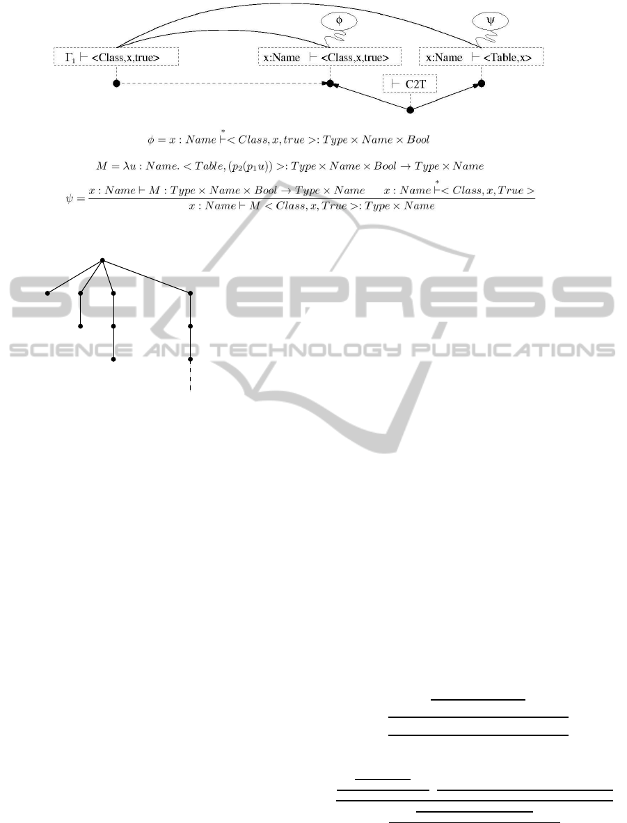
Figure 4: Example of a rule.
... ...
Figure 5: Example of ω-tree defined by the term
L(Rec
Nat→T
ω
(0)(λx
Nat
λy
T
ω
.S(y))). The length of the n-th
branch is n.
subtype into the elements of the supertype. It is com-
mon knowledge that the representation of the ele-
ments of a datatype is often changed when we pass
to a larger datatype, even if from mathematical point
of view it is merely an inclusion.
In coercive subtyping the subtyping relation A <
B is interpreted as existence of a certain definable
term c : A → B, with motivation of giving operational
semantics to calculi with subtyping and inheritance
(see, e.g., (Breazu-Tannen et al., 1991)).
In practice, certain “basic coercions” are defined
and other coercions are derived using appropriate
rules. For example, to the transitivity of subtyping
relation corresponds composition of coercions, from
two subtyping relations A < B and C < D one can de-
rive B → C < A → D, respectively, from the coercions
c
1
: A → B and c
2
: C → D one may derive a coercion
c : (B → C) → (A → D).
In the calculus with inductive types basic coer-
cions are usually certain coercions between inductive
types, for example the type Bool = Ind(α){T : α|F :
α} is the subtype of Nat = Ind(α){0 : α|S : α → α}
(with coercion c(T) = S(0) : Nat, c(F) = 0 : Nat).
The set of coercions may be represented by an
acyclic attributed graph where attributes of the nodes
represent corresponding inductive types. To do that
we may use free variables, e.g., to represent the type
A we take the axiom x : A ⊢ x : A as the attribute. Two
nodes corresponding to the types A and B are con-
nected by an arc if the types are in subtyping relation,
and the attribute of this arc is the coercion ⊢ c : A → B
(coercion terms representing basic coercions have no
free variables).
The set of coercions is coherent if composition of
coercion terms along two paths with the same source
and target is equal. The graph is completed to transi-
tive closure (concerning the attributes, coherence per-
mits to do it without contradiction). Practical useful-
ness of this is clear, since the coercions “implement-
ing” the subtyping relation can be directly taken from
the graph.
One of the main results obtained in (Soloviev and
Luo, 2001) was that coherence of the set basic coer-
cions implies coherence of the set of all derived coer-
cions. The main consequence was that the subtyping
extension of the consistent type theory without sub-
typing remains consistent.
Here we shall consider as an example two graph-
rewriting rules (besides already mentioned transitiv-
ity) that may be used to extend already obtained co-
ercion graph. They include the following derivations
used to define new coercions.
d =
x : A
∗
⊢ x : A
x : A,z :C ⊢ x : A
x : A ⊢ λz : C.x :C → A
⊢ λx : A.λz : C.x : A → (C → A)
d
′
=
∗
⊢ c : A → B
z :C ⊢ c : A → B
f : C → A, z :C ⊢ c : A → B
f : C → A, z :C ⊢ f : C → A f : C → A,z :C ⊢ z : C
f : C → A, z :C ⊢ fz : A
f : C → A,z :C ⊢ c( f z) : B
f : C → A ⊢ λz : C.(c( fz)) : C → B
⊢ λ f : C → A.λz : C.(c( fz)) : (C → A) → (C → B)
Here in fact d is an ordinary derivation and d
′
is a
partial derivation, active leaves (we refer to Ap-
IncorporatingProofsinaCategoricalAttributedGraphTransformationSystemforSoftwareModellingandVerification
69

c
4
d’
c
3
[A] [B]
→ A] [C → B]
c
2
c
1
c
3
[A] [B]
[C → A] [C → B]
c
2
c
1
[C
Figure 7: Rule 2.
x:A x:A
x:A x:A A→u:C A→u:C
λx:A λy:C.x:A → (C → A)
d
Figure 6: Rule 1.
pendix) are labeled by ∗. If A,B,C are considered
as the metavariables for arbitrary types and c as a
metavariable for arbitrary coercions, then we have
schemas of (partial) derivations instead of concrete
(partial) derivations. The instances will be obtained if
we take, e.g., Bool instead of A, Nat instead of B and
C, and concrete coercion c : Bool → Nat mentioned
above.
Of course, other rules to introduce new coercions
are possible, for example, a “contravariant” rule to
pass from A < B to B → C < A → C and the rules
for product types A∧ B.
Below we give an example of graph transforma-
tions using d and d
′
to define computation functions.
The rules are given in Fig. 6 and 7. In Fig. 7,
[A] denotes x : A ⊢ x : A, [B] denotes x
′
: B ⊢ x
′
: B
etc., c
1
denotes some coercion ⊢ c
1
: A → B, c
2
de-
notes ⊢ λx : A.λy : C.x : A → (C → A), c
3
denotes
λ.x
′
: B.λy
′
: C.x
′
: B → (C → B), and c
4
denotes
⊢ λf : C → A.λz : C.(c( fz)) : (C → A) → (C → B).
In Fig. 7 the left side may be assumed to be already
obtained by applications of the first rule
7
.
6 CONCLUSIONS
The aim of this paper was to generalize our previously
defined graph transformation system . As in (Boisvert
et al., 2011a), it is based on the SPo approach and its
main originality concerns the use of a partial deduc-
tions to express attribute computations. Type theory
7
The labels added using pairing may be used to avoid
repeated application of transformation rules to the same ar-
guments.
incorporates both λ-calculus and reductions as com-
putational mechanism, and has at the same time de-
duction rules for typing. The use of inductive types
permits to include user-defined datatypes, as in many
modern programming languages, and recursion over
these types.
That gives to our approach a great expressive
power that permit to manage classical model transfor-
mations like UML to Relational databasemodel trans-
formation, and also more sophisticated examples like
computation on functions, on infinite data structures,
or on proofs.
At the same time, thepresence of proofspermits to
establish connection between development and trans-
formation of software models and software certifica-
tion and verification.
Theoretically speaking, the SPo approach neces-
sitates the definition and the construction of a weak
pushout when dealing with attributes. A solution is
presented in this paper. In comparison with our pre-
vious papers, we presented a more powerful way to
describe transformation of attributes, using not only
computation with λ-terms but deduction rules.
The possible domains of applications include all
usual applications of graph transformations, e.g., ver-
ification and model transformations in software engi-
neering. Note that thanks to the approach described
above it is now possible to deal with certain infinite
models. More “tight” relationship between computa-
tion, graph structure and proofs will permit also the
pursuit of much more specific goals, in particular in
the domain of computer-assisted reasoning and veri-
fication (Luo, 1994),(Soloviev and Luo, 2001).
As a principal example of deductive system based
on type theory we considered in this paper the sim-
ply typed λ-calculus with inductive types and pairing.
All the constructions, though, can be easily modified
to be used in case of higher order and dependent type
systems in proof assistants, as well as for purely logi-
cal systems and applications.
A former experiment (Tran et al., 2010) of imple-
mentation in Haskell language constitutes the basis
for building a sofware environment devoted to model
MODELSWARD2013-InternationalConferenceonModel-DrivenEngineeringandSoftwareDevelopment
70

transformations using our new approach. This is a
natural practical extension of our current work.
REFERENCES
Baar, T., Strohmeier, A., Moreira, A. M. D., and Mellor,
S. J., editors (2004). UML 2004 - The Unified Mod-
elling Language: Modelling Languages and Applica-
tions. 7th International Conference, Lisbon, Portugal,
October 11-15, 2004. Proceedings, volume 3273 of
LNCS. Springer.
Barendregt, H., van Eekelen, M., Glauert, J., Kennaway, J.,
Plasmeijer, M., and Sleep, M. (1997). Term graph
rewriting. PARLE Parallel Architectures and Lan-
guages Europe, pages 141–158.
B´ezivin, J., Rumpe, B., Sch¨urr, A., and Tratt, L. (2005).
Model transformations in practice workshop. In MoD-
ELS Satellite Events, pages 120–127.
Boisvert, B., F´eraud, L., and Soloviev, S. (2011a). Typed
lambda-terms in categorical attributed graph rewrit-
ing. In 2nd WorKshop on Algebraic Methods in
Model-Based Software Engineering TOOLS 2011,
June 30th, 2011, Zurich, Switzerland . Electronic Pro-
ceedings in Theoretical Computer Science.
Boisvert, B., F´eraud, L., and Soloviev, S. (2011b). Typed
lambda-terms in categorical graph rewriting. In The
International Conference Polynomial Computer Alge-
bra, April 18-22, Saint-Petersburg, Russia, Euler In-
ternational Mathematical Institute.
Boisvert, B., F´eraud, L., and Soloviev, S. (2012). Graph
Transformations, Proofs, and Grammars. In Int. Conf.
Phylosophy, Mathematics, Linguistics, Aspects of In-
teraction, May 22-25, Saint-Petersburg, Russia, Euler
International Mathematical Institute.
Breazu-Tannen, V., Coquand, T., Gunter, C., and Scedrov,
A. (1991). Inheritance and implicit coercion. Infor-
mation and Computation, 93:172–221.
Bundy, A. (1988). The use of explicit plans to guide induc-
tive proofs. In Luck, E. and Overbeek, R., editors,
Proceedings of the 9th International Conference on
Automated Deduction (CADE), number 310 in LNCS,
pages 111–120. Springer, Argonne.
Chemouil, D. (2005). Isomorphisms of simple inductive
types through extensional rewriting. Math. Structures
in Computer Science, 15(5):875–917.
Combemale, B., Thirioux, X., and Baudry, B. (2012). For-
mally Defining and Iterating Infinite Models. In
France, R., Kazmeier, J., Atkinson, C., and Breu, R.,
editors, Proceedings of the 15th international con-
ference on Model driven engineering languages and
systems (MODELS’12), volume 7590 of LNCS, pages
119–133, Innsbruck, Austria. Springer.
Diestel, R. (2010). Graph Theory. Springer-Verlag, fourth
edition.
Ehrig, H. (1978). Introduction to the algebraic theory of
graph grammars (a survey). In Graph-Grammars and
Their Application to Computer Science and Biology,
pages 1–69.
Ehrig, H., Ehrig, K., Prange, U., and Taentzer, G. (2006a).
Fundamentals of Algebraic Graph Transformation
(Monographs in Theoretical Computer Science. An
EATCS Series). Springer-Verlag New York, Inc., Se-
caucus, NJ, USA.
Ehrig, H., Padberg, J., Prange, U., and Habel, A. (2006b).
Adhesive high-level replacement systems: A new cat-
egorical framework for graph transformation. Fun-
dam. Inf., 74(1):1–29.
Gentzen, G. (1934-35). Untersuchungen ¨uber das logische
Schliessen. In I, II, Math. Z. 39, pages 176–210, 405–
443.
Kleene, S. C. (1952). Permutability of inferences in
Gentzen’s calculi LK and LJ. Mem. Amer. Math. Soc.,
pages 1–26.
L¨owe, M., editor (1993). Algebraic approach to single
pushout graph transformation, TCS, volume 109.
Luo, Z. (1994). Computation and Reasoning: A Type The-
ory for Computer Science. International Series of
Monographs on Computer Science. Oxford University
Press, USA.
Luo, Z. (2008). Coercions in a polymorphic type system.
Math. Structures in Computer Science, 18(4):729–
751.
Orejas, F. (2011). Symbolic graphs for attributed graph con-
straints. J. Symb. Comput., 46:294–315.
Rebout, M. (2008). Une approche cat´egorique unifi´ee pour
la r´ecriture de graphes attribu´es. PhD thesis, Univer-
sit´e Paul Sabatier, Toulouse, France.
Rebout, M., F´eraud, L., Marie-Magdeleine, L., and
Soloviev, S. (2011). Computations in Graph Rewrit-
ing: Inductive types and Pullbacks in DPO Approach.
In Szmuc, T., Szpyrka, M., and Zendulka, J., editors,
Advances in Software Engineering Techniques, CEE-
SET 2009, Krakow, Poland, October 2009, volume
7054 of LNCS, pages 150–163. Springer-Verlag.
Rebout, M., F´eraud, L., and Soloviev, S. (2008). A Unified
Categorical Approach for Attributed Graph Rewrit-
ing. In Hirsch, E. and Razborov, A., editors, Interna-
tional Computer Science Symposium in Russia (CSR
2008), Moscou 07/06/2008-12/06/2008, volume 5010
of LNCS, pages 398–410. Springer-Verlag.
Rozenberg, G., editor (1997). Handbook of Graph Gram-
mars and Computing by Graph Transformations, Vol-
ume 1: Foundations. World Scientific.
Soloviev, S. and Luo, Z. (2001). Coercion completion and
conservativity in coercive subtyping. Annals of Pure
and Applied Logic, 113–1:297–322.
Taentzer, G., Ehrig, K., Guerra, E., Lara, J. D., Leven-
dovszky, T., Prange, U., Varro, D., and et al. (2005).
Model transformations by graph transformations: A
comparative study. In Model Transformations in Prac-
tice Workshop at Models 2005, MONTEGO, page 5.
Tran, H. N., Percebois, C., Abou Dib, A., F´eraud, L., and
Soloviev, S. (2010). Attribute Computations in the
DPoPb Graph Transformation Engine (regular paper).
In GRABATS 2010, University of Twente, Enschede,
The Netherlands, 28/09/2010-28/09/2010, page (elec-
tronic medium), http://www.utwente.nl/en. University
of Twente.
IncorporatingProofsinaCategoricalAttributedGraphTransformationSystemforSoftwareModellingandVerification
71

APPENDIX
Typed λ-Calculus with Inductive Types
The system of λ-calculus in this paper is the simply
typed λ-calculus with surjective pairing, terminal
object and inductive types. For details see (Chemouil,
2005), here we recall the principal definitions con-
cerning this system that will be named T in the other
sections of this paper.
Definition 6.1. Types are either atomic types or de-
fined by using a type constructor.
Atomic types are:
• the constant type ⊤;
• a finite or infinite set S = {α,β,...} of type vari-
ables;
Type constructors are:
• → for functional types, which constructs A → B
for any types A and B
• × for product types, which constructs A × B for
any types A and B
• Ind, defined as follows: let C be an infinite set of
introduction operators ( constructors of elements
of inductive types), with C ∩ S = ∅. an inductive
type with n constructors c
1
, . .., c
n
∈ C , each of
them having the arity k
i
(with 1 ≤ i ≤ n), has the
form:
Ind(α){c
1
: A
1
1
→ ... → A
k
1
1
→ α;
... ;
c
n
: A
1
n
→ ... → A
k
n
n
→ α},
Here, every A ≡ A
1
i
→ ... → A
k
i
i
→ α is an induc-
tive schema, i.e., A
j
i
is:
– either a type not containing α;
– or a type of the form A
j
i
≡ C
1
→ ... → C
m
→ α,
where α does not appear in any C
ℓ∈1..m
(such
A
j
i
are called strictly positive operators).
Here Ind(α) binds the variable α.
Example 6.1. (Definition of types Bool, Nat and T
ω
,
the type of ω-trees.)
F
n
= Ind(α){c
1
: α| ... |c
n
: α}
Bool = Ind(α){T : α|F : α}
Nat = Ind(α){0 : α| S : α → α}
T
ω
= Ind(α){0
ω
: α| S : α → α|L
ω
: (Nat → α) → α}.
Definition 6.2. Let V be an infinite set of variablesV
(with V ∩S ∩C = ∅). The set of λ-terms is generated
by the following grammar rules:
M ::= c|R
B,D
|x|(λx : B· M) | (M M) | < M M >
where x ∈ V , c ∈ C , B and D are arbitraty types, and
R
B,D
is the standard recursion operator (for details,
see (Luo, 1994), (Chemouil, 2005)).
All terms and types are considered up to α-
conversion, i.e., renaming of bound variables. Con-
text Γ is a set of term variables with types x
1
:
A
1
,...,x
n
: A
n
(x
1
,...,x
n
distinct). Γ,∆ denotes the
union of contexts Γ,∆ (we assume that Γ, ∆ have no
common term variables). The expression Γ ⊢ M : A is
called typing judgement (or sequent). Its meaning is
“term M has type A in the context Γ”.
Definition 6.3. Here are the following typing axioms
and rules for the terms defined above (A, B,D denote
arbitrary types, Γ arbitrary context).
Axioms.
• Γ,x : A ⊢ x : A, Γ ⊢ 0 : ⊤;
• For each inductive type C = Ind(α){c
1
:
A
1
|...|c
n
: A
n
} and 1 ≤ i ≤ n
Γ ⊢ c
i
: A
i
[B/α]
(for example, if C = Nat, we shall have Γ ⊢ 0 : Nat
and Γ ⊢ S : Nat → Nat);
• For C as above and any type D the axiom
8
:
Γ ⊢ R
C,D
:ϒ
C
(A
1
,D) → ... → ϒ
C
(A
n
,D) → C → D.
Typing Rules.
Γ ⊢ M : A Γ ⊢ N : B
Γ ⊢< M N >: A× B
(pair)
Γ ⊢ M : A× B
Γ ⊢ p
1
M : A
(p
1
)
Γ ⊢ M : A× B
Γ ⊢ p
2
M : B
(p
2
)
Γ,x : A ⊢ M : B
Γ ⊢ (λx : A · M) : A → B
(λ)
Γ ⊢ M : A → B Γ ⊢ N : A
Γ ⊢ (M N) : B
(app)
Remark 6.1. (i) The constant R
C,D
is called the re-
cursor from C to D. Notice that applying it (using
the rule app) to the terms M
1
: ϒ
C
(A
1
,D),...,M
n
:
ϒ
C
(A
n
,D) we define the function R
C,D
M
1
...M
n
: C →
D. The following derived rule is often included:
Γ ⊢ M
i
: ϒ
C
(A
i
,D)(1 ≤ i ≤ n)
Γ ⊢ (R
C,D
M
1
... M
n
) : C → D
(elim)
(ii) Usually the following structural rules are in-
cluded in T (they are admissible w.r.t. other rules):
Γ ⊢ M : B
Γ,x : A ⊢ M : B
(wkn)
Γ,x : A, x
′
: A ⊢ M : B
Γ,x : A ⊢ [x/x
′
]M : B
(contr)
8
ϒ
C
(A,D) are certain auxilliary types used to define re-
cursion from C to D. They correspond to the types of func-
tions that appear in standard recursive equations overC. For
example, if C = D = Nat and A = Nat → Nat (the type of
successor S), then ϒ
Nat
(A,Nat) = Nat → Nat → Nat.
MODELSWARD2013-InternationalConferenceonModel-DrivenEngineeringandSoftwareDevelopment
72

Γ ⊢ N : A Γ,x : A ⊢ M : B
Γ ⊢ [N/x]M : B
(subst)
Here [N/x] denotes substitution with renaming of
bound variables to avoid capture.
Normalization and Equality. The terms of the sys-
tem T are considered up to equality generated by
conversion relation. The α-conversion (renaming
of bound variables) was already mentioned. Other
conversions are
9
: (i) β-conversion (λx : A.M)N =
[N/x]M; (ii) η-conversion λx : A.(Mx) = M (where
x must not be free in M); (iii) and ι conversion for
recursion. The ι-conversion corresponds to one step
in recursive computation. It applies to the terms of
the form (R
C,D
M
1
...M
n
)(c
i
N), i.e. when the func-
tion defined by recursion applied to the term begin-
ning by one of the introduction operators. For exam-
ple, for (R
Nat,Nat
ag)0 →
ι
a and (R
Nat,Nat
ag)(Sn) →
ι
(R
Nat,Nat
ag)((gn)(Sn)) (here a : Nat is “initial value”
and g : Nat → Nat → Nat defines inductive step. The
exact general definition may be found in (Chemouil,
2005), p.884.
T is confluent and strongly normalizing with re-
spect to βηι-reductions (directed conversions). De-
tailed description and normalization theorems for T
can be found in (Chemouil, 2005). Thus, the equiv-
alence relation on terms based on conversion (often
called βηι-equality) is decidable.
Proof Trees and Partial Proofs
An inference rule in proof theory is a couple
P
C
where
P is a list of premises, possible subject to some con-
straints. As examples one may take the rules of the
system T above. Usually in proof theory the presen-
tation of rules is schematic, that is, the metavariables
like Γ,∆ are used to represent arbitrary contexts, A,B
to represent arbitrary types etc. The presentation be-
low is generic, i.e., all the definitions can be modified
to accomodate a change of logical system, if only the
system has tree-form derivations build by application
of deduction rules to their premises.
Trees are a special case of graphs, and proof trees
are a special case of attributed graphs, but in any
case the trees below should be considered as part of
metatheory and not the objects of the category of at-
tributed graphs defined in this paper. Applications
of trees to computations and data structures are usu-
ally straightforward, in difference from graphs in gen-
eral
10
. Our generalization of the definition of graph
9
We omit the contexts and types of terms.
10
The possibility to “embed” them into this category
seems obvious, but to our opinion it may be considered as
an invitation to study a hierarchy of graphs and attributes
transformation systems is based on the notion of par-
tial proof. Below the reader may assume that the par-
tial proofs are taken in the system T described above
but the definition will apply to any other deductive
system with appropriately defined derivable objects.
According to standard definitions (cf. (Diestel,
2010)), a tree is a connected directed acyclic graph
J = (V,E) in which a single node is designated as root
and there is a unique path from the root to any other
node. If (x,y) ∈ V, we say that y is a child of x and y is
the parent of x. A leaf has no children. Since J has no
directed cycles, the transitive closure E
∗
of E defines
a partial strict order on V. There is a path from x to y
in J iff (x,y) ∈ E
∗
.
An ordered tree is the tree where outgoing edges
of any v ∈ V are numbered 0, 1,.... Thus, to any
(x,y) ∈ E
∗
corresponds a unique sequence of natu-
ral numbers. The lexicographic ordering of these se-
quences beginning at the root r permits to extend this
partial order to the unique linear order on V. In par-
ticular there is the natural ordering of the leaves.
The definitions below are modified definitions
from (Bundy, 1988) adapted to our case.
Definition 6.4. A partial proof is an ordered tree with
the following properties: (i) each node is labelled
with a sequent and the rule of inference which is ap-
plied to this sequent (backwards) to produce the (la-
bels of) the node’s children; (ii) the final sequent (or
the goal) is the sequent at the root of the tree; (iii) for
the leaves, no rule of inference is specified; (iv) we
shall further distinguish “active” and “parameter”
leaves. Active leaves are marked by ∗.
Our purpose is to use partial proofs for attribute
transformations, and thus, the difference between ax-
ioms and other sequents is not relevant. In some cases
we may impose additional restrictions, e.g., that the
parameter leaves are axioms or that all leaves have
derivable sequents as labels.
The use of partial proofs instead of λ-terms to rep-
resent computation functions permits more flexibility
concerning the choice of equality in the category of
graph transformations. The definitions and results be-
low will be valid for any equality (equivalence rela-
tion) on the set of sequents (logical formulas, judge-
ments). Usually (but not necessarily) the judgements
of the system T are considered up to βηι-equality.
Another choice may be syntactic (graphic) equality
of terms and types (with γ and Γ
′
equal as sets).
Next notion we are going to define is the equality
of partial proofs. In fact, the main requirement is that
the good properties of composition must be assured.
with alternating layers. The possibility seems interesting
but it is out of scope of this paper.
IncorporatingProofsinaCategoricalAttributedGraphTransformationSystemforSoftwareModellingandVerification
73

Definition 6.5. Partial proofs are equal if they have
the same number of active leaves, the labels of corre-
sponding active leaves (in order defined by the trees)
and the labels of two roots are equal
11
.
The notion of composition of partial proofs is in-
spired by the notion of composition of multivariable
functions.
Definition 6.6. Let l
1
< ... < l
k
be all active leaves
(see definition above) of the partial proof P. Let P
1
,...,
P
k
be partial proofs and r
1
,...,r
k
their roots. Let
for all i, 1 ≤ i ≤ k the labels of l
k
and r
k
be equal.
The composition P ∗ (P
1
,...,P
k
) is obtained by iden-
tification of each l
i
with its label and r
i
with its la-
bel (assuming other nodes disjoint). Order relations
are extended to the new tree in natural way. The ac-
tive leaves are now the union of the active leaves of
P
1
,...,P
k
and the root is the root of P.
The result is another partial proof. This composi-
tion is associative w.r.t. the equality defined above.
Definition 6.7. The canonical identity partial proof
for the sequent (formula, judgement) S is the tree with
one node (which is the root and the one active leaf at
the same time) that has S as its label.
Schemas of Partial Proofs
It is common in proof theory to use axiom and rule
schemas instead of individual axioms and rules. In
the schemas the meta-variables may be used. The for-
mulations of axioms and rules of the system T above
are schematic. There may be metavariables of differ-
ent kinds, e.g., metavariables for terms, contexts, and
even for arbitrary variables as in the axiom schemas
or the rule (λ) above
12
.
Definition 6.8. (Partial Proof Schema.) A partial
proof schema is an ordered tree with the following
properties: (i) each node is labelled with a meta-level
sequent. (ii) each node except the leaves is labeled
also with the rule of inference which is applied to this
sequent (backwards) to produce the node’s children
(and the children of course must be the meta-level se-
quents matching the premises of this rule). (iii) the
final meta-level sequent (or the goal) is the meta-level
sequent at the root of the tree, some of the leaves are
marked as active by ∗.
11
An alternative definition would be to require the equal-
ity of the whole ordered trees and all corresponding labels.
12
Essentially, this practice is similar to the use of non-
terminals in the formal grammars.
MODELSWARD2013-InternationalConferenceonModel-DrivenEngineeringandSoftwareDevelopment
74
