
Low Cost Adaptive Optics Testbed for Small Telescopes
Manuel Cegarra and Andrew Lambert
School of Engineering and IT, UNSW Canberra, Northcott Drive, Canberra ACT 2600, Australia
Keywords: Atmosphere Turbulence, Deformable Mirror, FPGA, Wavefront Sensor.
Abstract: The aim of this work is the development of a low cost Adaptive Optics system that can be used as a testbed
for laboratory research installed on a small telescope. An optical system has been designed supported in a
mechanical structure, and a control system has been developed and installed in a FPGA reconfigurable
platform. Particular premises specific to small telescopes have been considered in the design and
development stages, such as the use of low cost optical and electronic components, and the portability and
lightness of the platform. Laboratory tests successfully validate that the whole control system can be
implemented in a low cost standalone FPGA device and that an optical subsystem mounted in a
configurable and lightweight structure can be used for laboratory test and telescope use.
1 INTRODUCTION
Adaptive Optics (AO) can be considered a technique
to compensate the aberrations in the wavefront of a
light beam that travels through a medium. One of its
main applications is astronomy, although it could be
also applied in, for instance, surveillance,
ophthalmology or microscopy. In the case of
astronomy, these aberrations are produced by the
atmospheric turbulence, due to terrestrial surface
heating.
AO doesn't have a long history. Its origins date
back around the 1950's. Firstly it was promoted by
astronomical associations and defence governmental
departments, and in the last 30 years has suffered a
rapid evolution, in part due to the enhancements
experimented by computer processing, sensors and
actuators, which are the three main technologies on
which adaptive optics is based (Tyson, 2000). In the
mid-90s AO systems were only in the planning
stages for the current big telescopes (with diameter
bigger than 3 metres).
Nowadays the high budget astronomy is strongly
dependant on AO systems. This sector of astronomy
comprises big telescopes in observatories spread all
over the world. Also, bigger telescopes (Extremely
Large Telescopes, ELT) from 20 to 100 metres in
diameter, are currently under construction. These
ones will require complex AO systems.
Less research has been performed in the medium
and low budget astronomy sector, which can be
considered formed by small research installations,
medium size observatories, universities and amateur
astronomy. In general terms, AO is expensive. It
consists of precise and well designed opto-
mechanical components, where alignment and
precision are fundamental issues, and the more
expensive the components, the better performance
the system will have, requiring a reasonable budget,
research work and engineering work in several
fields, as electronics, optics, or mechanics.
The hypothetical performance of an AO system
in a small telescope has to be considered. In this
kind of telescope, less photons are introduced in the
system and resolution is lower, which could raise
some doubts about the advantages of the use of AO
systems in this sector.
However, currently some commercial AO
systems for small telescopes are available such as
the commercialized by Santa Barbara
(http://www.sbig.com/Adaptive-Optics/) and Stellar
Products (http://www.stellarproducts.com/). These
systems are intended to correct low order local
atmospheric effects. Other companies have
developed more versatile solutions
(http://www.okotech.com/ao-systems,
http://www.bostonmicromachines.com/aosolutions.h
tm).
The concept of a low cost AO system for its use
in medium and small size telescope has been
developed by different authors, proposing various
optic and computer control configurations
45
Cegarra M. and Lambert A..
Low Cost Adaptive Optics Testbed for Small Telescopes.
DOI: 10.5220/0004337900450051
In Proceedings of the International Conference on Photonics, Optics and Laser Technology (PHOTOPTICS-2013), pages 45-51
ISBN: 978-989-8565-44-0
Copyright
c
2013 SCITEPRESS (Science and Technology Publications, Lda.)

(Aceituno, 2009); (Loktev et al., 2008); (Teare et al.,
2006).
Although the control of first AO systems were
designed using traditional CPU (Central Processing
Unit) architectures, advances in computer
processing, with the emergence of other kind of
electronic devices as Field Programmable Gate
Array (FPGA) or Graphics Processing Unit (GPU)
changed dramatically the approach to this issue.
FPGA technology was considered some years ago as
an option to implement the control algorithm, due to
its inherent pipeline and parallel design possibilities,
low cost, and high speed architectures. FPGA
devices can be easily reprogrammed, providing a
high degree of flexibility in the development phase.
The reduced size of devices nowadays has decreased
the overall size of electronic architectures, opening
possibilities to more lightweight AO systems, which
could be used in small telescopes.
During the last 10 years several research teams
have worked in the proposal of electronic
architectures which use FPGA as central processing
unit (Peng et al., 2008); (Rodriguez-Ramos et al.,
2006); (Saunter et al., 2005). In AO control several
stages are involved, being some of them of high
computational requirements, as VMM (Vectorial
Matrix Multiplication), in order to obtain the
reconstructed wavefront. Reconstruction algorithms
require an iterative process, thus making them
appropriate for pipeline and parallel processing, so
they are suitable for implementation in Digital
Signal Processor (DSP), GPU and FPGA devices.
Research efforts in control systems have mainly
targeted high-end FPGA devices, because their use
was intended for AO systems installed in big
telescopes, where the cost of the electronic
architecture was a minor problem in the overall cost
of the project. Nevertheless, some authors have
focused in low cost FPGA devices and have proved
that latency times can also be reduced, even with
these kind of devices, and have opened the
possibility to their use as a standalone device within
an AO system (Kepa et al., 2008).
2 AO FUNDAMENTALS
2.1 Atmosphere Turbulence
Atmosphere turbulence is the main parameter to
limit the resolution of Earth based telescopes. Air
masses of different sizes moving at various speeds
produce variations in the refraction index of the
incoming wavefronts. As a consequence, these
variations modify the intensity and phase of the
wavefront, resulting in scintillation and blurry
images. One way to measure the turbulence
extension is through the ratio D/r
0
, where D is the
diameter of the telescope and r
0
is the Fried
coherence length, which is a parameter describing
the spatial extent of the turbulence. In high
mountains, where air is less turbulent, this ratio
scales with telescope diameter. Nevertheless, in
poorer air, small telescopes have similar D/r
0
as
large ones.
Current AO systems reach boundaries in the
isoplanatic area, which is the region of the
observation field where relative changes in the
atmospheric turbulence can be deprecated. Due to
this limitation, in recent years some researchers have
focused in the way to correct aberrations beyond the
isoplanatic area, that is, in wide field of view, and
solutions as MCAO (Multiple Conjugate Adaptive
Optics) and MOAO (Multiple Object Adaptive
Optics) have arisen.
MOAO, MCAO, or hybrid solutions increase the
number of optical elements in the AO systems,
turning it into a more complicated system to design,
to control or to manage. While this is of some
importance in a big telescope, in a low cost small
system this is a big issue, so a study and assessment
of other options in these systems needs to be
addressed. Some authors have proposed the use of a
software approach to extent the isoplanatic patch, as
RNN (Recurrent Neural Network), removing the
need of an optical solution (Weddell, 2010).
2.2 AO System
A traditional AO system is composed of three main
components: control system, wavefront sensor
(WFS) to measure the aberrations, and deformable
and tip-tilt mirrors to correct them mechanically.
The control system, which is implemented in CPU
or other dedicated hardware resource, obtains gain
and phase information of the incoming wavefront
from the sensor, and processes it in order to obtain
signals that will be applied to the actuators of the
deformable and tip-tilt mirrors, to reproduce a
conjugate to the aberrated wavefront. This is a real
time closed loop process.
In order to achieve the real time requirement of
the feedback loop, the whole computation time has
to be within the variation rate of the refraction index
distortions introduced by atmosphere, typically 10
ms for well sited telescopes, but potentially much
shorter for the situations considered herein.
PHOTOPTICS2013-InternationalConferenceonPhotonics,OpticsandLaserTechnology
46
There is a balance to ensure maximum possible
light gets to the science camera. There are several
kinds of wavefront sensors based in different
techniques, as Shack-Hartmann, pyramidal or
curvature. One of the more widespread, due to its
ease of implementation is the Shack-Hartmann. In
this sensor the beam goes through a lenslet array,
which divides it into several small beams
corresponding with each of the subapertures. The
detector (usually a CMOS (Complementary Metal
Oxide Semiconductor) or CCD (Charged Coupled
Device) image sensor) is positioned in the focal
plane of these beams. The positions of the focused
beams deviate when an aberrated beam is introduced
in the system, with respect the positions obtained
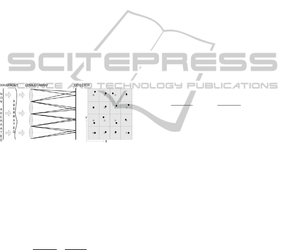
with a non-aberrated beam. A measurement of the
local slopes of the beam phase for each subaperture
can be obtained from these deviations, as shown in
figure 1, where gray dots and black dots represents
centroids from a non-aberrated and an aberrated
wavefront respectively.
Figure 1: (Left) Shack-Hartmann wavefront sensor.
(Right) Movement of sensor image within lenslet array.
Calculation of the deviation could be performed
by several algorithms. CoG (Center of Gravity)
calculation is a straightforward method to obtain
these deviations (Fusco et al., 2006). Although it has
some limitations with real spots, it is well suited for
the purpose of this work.
If W(x,y) is the wavefront captured in the
detector with respect to axis x and y, by geometry
these differences can be related with the
corresponding slopes in each of the subapertures.
,
Δ,
f
(1)
In equation 1 this relation is expressed in x axis,
where ∆x(x,y) is the gradient in the centroid position
in x axis for a subaperture, and f is the focal distance
of each of the lens of the lenslet array. A similar
equation exists for y gradients.
2.3 Reconstruction Process
The control system receives the positions of the
focused beams of each subaperture from the
detector, and its aim is to produce the signals that
will be sent to the actuators of the tip-tilt and
deformable mirrors, with minimum latency.
To reconstruct the aberrated wavefront, a modal
approach can be used, whereby W(x,y) can be
expressed as a weighted sum of Zernike
polynomials, with each of terms representing a
different optical aberration, as follows:
,
.
(2)
In equation 2, term w
i
represents the Zernike
coefficients of each of the aberrations, Z
i
(x,y) the
Zernike polynomials, and N the number of
aberrations polynomials considered.
From equations (1) and (2), the gradients of each
of the subapertures can be related with a weighted
sum of Zernike polynomials, as follows:
Δ,
f
,
(3)
Considering all the subapertures in both axes,
equation (3) can be expressed in matrix form as
follows:
(4)
If k is the number of subapertures, in equation (4) ∆
is the gradients matrix with 2k × 1 dimensions, Z is
the partial derivative of Zernike polynomial matrix
in both axes of dimensions 2k × N, and W is the
Zernike coefficients matrix of dimensions N × 1.
In order to obtain the Zernike coefficients from
equation (4), least square estimation method could
be applied to obtain the pseudoinverse matrix of Z,
resulting in equation (5).
;
(5)
In equation (5) C is called the calibration matrix,
with dimensions N × 2k.
In order to obtain the signals to be applied to the
mirrors actuators, the influence functions have to be
derived, each of them representing the bidimensional
profile generated for each of the actuators. Each of
the actuators will have a value to represent each of
the Zernike coefficients. The matrix which relates
these parameters is called influence matrix, I.
Finally, from equation (5) and the influence
matrix, the voltages required by the actuators to
reproduce a specific wavefront can be obtained as
LowCostAdaptiveOpticsTestbedforSmallTelescopes
47

follows:
(6)
In equation (6) V is the voltages actuator matrix, and
j is the number of actuators.
3 AO PLATFORM
In order to assess the feasibility of a low cost AO
system to be implemented, a mechanical support has
been developed, with an attached optical setup.
Below is a detailed description of each subsystem,
mechanical support, optical setup and control
system.
3.1 Mechanical Support
The first stage is the definition of the mechanical
constraints that affect the system. The structure had
to be lightweight, thus having the lowest impact as
possible in the overall telescope weight together
with the AO system, in order to ease the balance of
the system. At the same time, the support at the
junction of optical structure with telescope rear port
had to be solid enough to support a weight which
will be around 10 kg, which is the expected average
weight of the AO system, including optical
components, electronic board and the structure itself.
The main aspect which needs to be addressed is that
it must have enough flexibility to accommodate
different optical components at different distances
between them for experimentation. Also the size of
the AO structure has to be small enough to be
considered portable.
The weight of the platform without optics and
electronic components is 4.5 kg, and the total
estimated weight is 10 kg. The dimensions of the
platform are 470 × 350 × 100 mm. Figure 2 shows
the 3D model of the AO system prototype.
3.2 Optical Setup
The optics subsystem is modelled to evaluate the
performance of the whole system in closed loop
under test conditions.
The laboratory test and validation conditions
evaluate the system with a laser light source,
optically aligned with the optical setup, so there is
no need to consider at this stage the tip-tilt
correction of the beam. Not considered yet are the
weak photon flux and the light incoherence of the
light coming from an astronomical source. The laser
light source generates a high intensity and
Figure 2: Mechanical testbed 3D model.
correctly aligned beam, to evaluate the capacity of
the optical system and generate a valid centroids
pattern, which will be used by the control system to
generate the appropriate signals for the deformable
mirror actuators.
Figure 3 shows the optical setup of the AO
system. All lenses of the optical setup are plano-
convex with 1" or 2" diameter, anti-reflection coated
for 350 to 700 nm and the substrate material is N-
BK7 (grade A). Flat mirrors have more than 90%
average reflectivity and flatness below 5λ/in
2
. Here
is a description of the components and main points
of the optical setup.
P1: Telescope emulation. A f/10 telescope has
been emulated with a HeNe Class 2 laser source,
with 0.5 mW output power, forming an image at F1.
Fi1: A neutral density filter is used to decrease
the laser intensity which could saturate the image in
the detector.
L1: Collimation lens with focal length 200 mm.
This lens collimates the beam to a diameter
appropriate to illuminate the deformable mirror
effective surface.
M1: A flat mirror which directs the beam to the
deformable mirror. In the next stage of the project
this mirror will be substituted by a tip-tilt mirror
system, to correct the first order aberrations of the
incoming beam.
M2: An OKO 30 mm 19-channel piezoelectric
deformable mirror. The beam encompasses the
effective surface of the mirror.
L2, L3: A Kepler telescope. Focal lengths of L2
and L3 are 100 mm and 50 mm respectively. This
telescope system selects the beam diameter which
will illuminate the lenslet array, resulting in different
number of centroids in the wavefront sensor. In
order to get this feature, L3 could be exchanged with
PHOTOPTICS2013-InternationalConferenceonPhotonics,OpticsandLaserTechnology
48
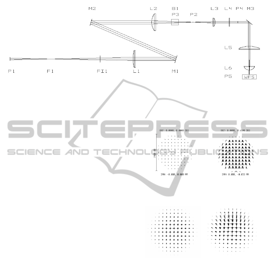
Figure 3: Optical setup. P1: position of the telescope. F1: focal plane of telescope. FI1: neutral density filter. L1:
collimation lens. M1, M3: flat mirrors. M2: deformable mirror. L2, L3: Kepler telescope. B1: beamsplitter. P2, P3: Focal
plane of corrected image. L4: lenslet array. P4: focal plane lenslet array. L5, L6: telecentric system. P5: WFS focal plane.
WFS: wavefront sensor.
lenses with different focal lengths.
B1: Beamsplitter to divide the incoming beam in
two parts, one used to generate the centroids, and the
other to register or visualize the corrected image in
the science camera (nitrocellulose pellicle
beamsplitter of 2" 45%R 55%T).
P2, P3: Focal plane of the corrected telescope
emulator image. P3 is the science camera, needed to
register the corrected images.
L4: Lenslet array. It consists on a plano-convex
set of 0.5 x 0.5 mm square array of lenses, and focal
distance 23 mm.
P4: Focal plane of the elements of the lenslet
array.
M3: Another flat mirror to adapt the optical
design to the mechanical constraints of the platform.
L5, L6: These two lenses comprise a telecentric
optical system. Focal lengths of L5 and L6 are 100
mm and 25.4 mm respectively. This system is used
to adapt the size of the incoming beams from the
lenslet array at the appropriate scale of the
wavefront sensor detector.
P5: Reimaged focal plane on the wavefront
sensor detector, which consists in a Pixelinx PL-
A741 monochrome camera with 1.3 megapixel
resolution (1280 × 1024), and 6.7 x 6.7 µm pixel
size.
Figure 4 shows the geometric image analysis in
the focal plane of the centroids, at 0 and 0.65
degrees input angle. Note the lateral shift in the
centroids positions with input angle, while figure 5
shows the image from the wavefront sensor camera
obtained in the lab from which the centroids can be
determined. The centroids shapes exhibit similar
distortion off-axis, compared to predicted in
simulation results shown in figure 4.
Figure 4: Spot diagram at 0 (left) and 0.65 (right) degrees
input angle.
Figure 5: Image captured by WFS camera containing spots
to be centroided on axis (left) and off axis (right).
3.3 Control System
In this section the control algorithm is discussed, and
simulation results comparing floating point and
fixed point precision are shown. Also experimental
results from implementation in the FPGA device are
presented.
3.3.1 Control Algorithm Architecture
The electronic top level architecture and the main
blocks with comprise the FPGA control board are
shown in figure 6.
LowCostAdaptiveOpticsTestbedforSmallTelescopes
49

Figure 6: Top level electronic architecture, showing the
relationships between the main blocks of the system.
The wavefront sensor is programmed into the
FPGA control board, in order to generate the
appropriate clock and data signals. The signals will
be obtained through the control algorithm, to send to
the high voltage deformable mirror drive board for
the voltages required by the deformable mirror.
The FPGA processes the signals provided from
the wavefront sensor block, and the signals to the
deformable mirror actuators will be serialized and
sent to the D/A converters on the drive board.
The control algorithm of the electronic
architecture has been programmed in VHDL
(VHSIC Hardware Description Language) and
implemented in a FPGA Spartan3E XC3S500E.
Figure 7 is an illustration of the block diagram of
the control algorithm implemented in the FPGA.
Mathematical operations are represented as light
gray blocks, while clear blocks represent preloaded
data in FPGA embedded or distributed RAM
(Random Access Memory). The DATA FLOW
CONTROL block (in dark gray) manages the data
flow along the process, generating control logic,
delays and the appropriated enable and reset signals
to each segment of the process.
3.3.2 Floating Point vs. Fixed Point
The FPGA shares resources in a time division
multiplexing process, taking advantage of the per
clock basis nature of the process, using pipeline
when is required. Parallel processing is performed in
the X and Y axis computation blocks where
appropriate, with the aim to get the minimum
latency time at the end of each frame processing.
In order to get high computation speed, FPGA
operations are performed with a fixed point
resolution. To assess the accuracy of the obtained
data, two models were designed in MATLAB, one
with double floating point resolution, and the other
with fixed point. In the whole computation process,
the selection of the number of bits for the fractional
part of the divisions is a key parameter which affects
both resolution and utilization of hardware FPGA
resources.
A synthetic image was created, in order to
generate centroids in random positions, which
affects all the Zernike modes considered. A 300 x
300 pixel image was created, subdivided in 10 x 10
subapertures, hence each of the subapertures consist
of 30 x 30 pixels squares. Nine Zernike modes were
considered, but not piston movement, resulting in
Zernike coefficients from W1 to W9.
Figure 8 shows the relative error in tip and tilt
modes of Zernike coefficients (W1 and W2), when
fixed point resolution with different number of bits
in the fractional part is selected, compared to
floating point precision. These differences have been
evaluated for three tip-tilt slope severity levels,
corresponding to 1 pixel, 7 pixels and 14 pixels
displacement of the centroids.
Figure 7: Blocks diagram of FPGA control algorithm.
PHOTOPTICS2013-InternationalConferenceonPhotonics,OpticsandLaserTechnology
50
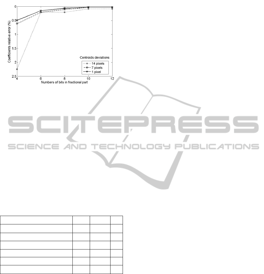
Figure 8: Error in W1 and W2 Zernike coefficients with
different number of bits in the fractional part, compared
with floating point precision.
Notice that error introduced by the use of fixed
point resolution with 10 bits or more in the fractional
part is independent of the number of extra bits.
Below 6 bits, the relative error increases more
dramatically. This analysis does not include PSF
(Point Spread Function) distortion.
The fixed point model with 10 bits in the
fractional part was synthesized in a Spartan 3E
XC3S500E and in table 1 is shown the FPGA
utilization summary, indicating that the control
system can be implemented in a low capacity FPGA.
Auxiliary tasks can be included.
Table 1: FPGA utilization summary, showing the
percentage of used resources in device.
Logic utilization Used Available %
Number of slice FlipFlop 6.231 9.312 67
Number of 4 input LUTs 3.693 9.312 40
Number of occupied slices 3.654 4.656 78
Number of RAMB16s 6 20 30
Number of BUFGMUXs 1 24 4
Number of MULT18x18SIOs 9 20 45
4 CONCLUSIONS
An AO platform has been developed for use with
small telescopes, and tested in the laboratory. The
optical configuration shows that with low cost
components a flexible light path could be built. The
whole control algorithm was implemented in a low
cost standalone FPGA, a Spartan3E XC3S500E,
without requiring extra computing devices. If more
computing operations, such as filters, were required,
the VHDL based code could be easily exported to a
more powerful FPGA device. Results from
simulation and implementation of the control
algorithm shows a correct behaviour with only 60
clock cycles latency from the last pixel of a frame
sent to the control system.
We are yet to examine the dynamic performance
of the AO control system, taking into account delays
in the mirror actuators and other parts of the system,
including a tip-tilt mirror control in the FPGA.
REFERENCES
Aceituno, J. (2009). PhD Thesis, Prototipo de sistema de
óptica adaptativa basado en un espejo deformable de
membrana para aplicación astronómica. Universidad
de Granada, Granada.
Fusco, T., Thomas, S., Nicolle, M., Tokovinin, A.,
Michau, V., & Rousset, G. (2006). SPIE 6272,
Advances in Adaptive Optics II, 627219.
http://www.sbig.com/Adaptive-Optics/. 14-10-2012.
http://www.stellarproducts.com/. 14-10-2012.
http://www.okotech.com/ao-systems. 14-10-2012.
http://www.bostonmicromachines.com/aosolutions.htm.
14-10-2012.
Kepa, K., Coburn, D., Dainty, J., & Morgan, F. (2008).
Measurement Science Review, 8(4), 87-93.
Loktev, M., Vdovin, G., & Soloviev, O. (2008). Paper
presented at the Proc. SPIE 7015, Adaptive Optics
Systems, 70153K, Marseille, France.
Peng, X., Li, M., & Rao, C. (2008). Paper presented at the
Proc. SPIE 7130, 71303Z.
Rodriguez-Ramos, L. F., Viera, T., Herrera, G., Gigante, J.
V., Gago, F., & Alonso, A. (2006). Art. no. 62723X.
Advances in Adaptive Optics II, Prs 1-3, 6272, U1326-
U1335.
Saunter, C. D., Love, G. D., Johns, M., & Holmes, J.
(2005). Proc. SPIE 6018, 60181G.
Teare, S. W., Martinez, T., Andrews, J.R. (2006). Art. no.
630609. Advanced Wavefront Control: Methods,
Devices, and Applications IV, 6306, 30609-30609.
Tyson, R. K. (2000). Introduction to adaptive optics /
Robert K. Tyson. Bellingham, WA: SPIE Press.
Weddell, S. J. (2010). A Thesis Presented for the Degree
of Doctor of Philosophy, New Zealand: University of
Canterbury.
LowCostAdaptiveOpticsTestbedforSmallTelescopes
51
