
Simulation Models for Grassland Ecosystem and
Inter-species Plant Competition: Interation in NetLogo
Ngoc Bich Dao, Arnaud Revel, Michel Menard and Abdallah El Hamidi
Laboratoire MIA, Universit
´
e de La Rochelle, La Rochelle, France
Abstract. In this article, we have first implemented El Hamidi, Garbey and Ali’s
nonlinear diffusion model of the competition of plants on the Netlogo platform.
In parallel with this partial differential equation (PDE) model, an agent based
diffusion model has been implemented to compare the structures of the two ap-
proaches. The multi-agent system (MAS) models how each individual grows up
[1] and is spatially diffused thanks to reproduction. Furthermore, El Hamidi’s
nonlinear diffusion model has been extended to the case of n species in a sys-
tem of inter-species plant competition. We have also studied how the inter/intra-
specific competition parameters impact the space distribution by computing the
surface ratios between species. Besides, terms representing resources have been
added to measure the effects of environmental parameters. Finally, we propose
a comparison between PDE and MAS approaches by identifying parameters of
both models that correspond to each other.
1 Introduction
Plants evolve along time following a predefined life cycle: birth, growth, maintenance,
sexual maturity, reproduction, death and decay. During these processes, plants alter the
composition of the surrounding environment. When simulating plants’ development
two main phenomena must thus be taken into account: the growth of each individual
and the diffusion of the population by reproduction. The growth and spread of plants
are influenced by many environmental parameters such as the presence of light, the dis-
persion of resources in the earth and in the air [2], the wind direction or strength, etc.
They are also influenced by parameters that depends on the plant properties such as the
seed weight, shape, the height of the plant from which the seed is diffused, etc. More-
over, dissemination of asexual plants is different from that of bisexual plants because
with the latter, the diffusion depends on the number of plants of different sexes which
are present in a given radius. The models studied in this article are only focused on the
case of asexual plants.
The first model we have implemented is a nonlinear diffusion model of the com-
petition of two plants [3]. This model is based on a diffusive PDE (partial differential
equation) implemented on the NetLogo platform with Neumann boundary conditions,
and a discretization of both time and space. We have also extended El Hamidi’s nonlin-
ear diffusion model to the case of n species in a system of inter-species plant compe-
tition. Moreover, we have studied how the inter/intra-specific competition parameters
impacts the space distribution by computing the surface ratios between species. In order
to measure the effects on plants of environmental parameters such as the dispersion of
Dao N., Revel A., Menard M. and El Hamidi A..
Simulation Models for Grassland Ecosystem and Inter-species Plant Competition: Interation in NetLogo.
DOI: 10.5220/0004347600200028
In Proceedings of GEODIFF 2013 (GEODIFF-2013), pages 20-28
ISBN: 978-989-8565-49-5
Copyright
c
2013 SCITEPRESS (Science and Technology Publications, Lda.)

resources in the earth and in the air, light and wind, terms representing resources have
been added. Two conditions have been considered: nonlinear isotropic and anisotropic
diffusion.
In parallel with the PDE model of two species, a diffusion agent based model has
been implemented to compare the structures of the two approaches. The multi-agent
system models how each individual grows up [1] and is spatially diffused thanks to
reproduction. Finally, we propose a comparison between PDE and MAS approaches by
identifying parameters of both models that correspond to each other. For instance, the
inter-species competition of the PDE model is performed by the local plant strategy of
space colonization.
2 Modeling Diffusion Species of a Prairie Ecosystem
2.1 Model of Nonlinear Diffusion of 2 Species with PDE
In recent years, the equation of diffusion-reaction in a competition system has been
widely used in bioinformatics and mathematics [4–6]. Based on the model of Volterra-
Lotka, [3] proposes this following model of diffusion:
u
t
− ε
1
div (Φ (v) ∇u) = u (α
1
− β
1
u − γ
1
v) , (x, y) ∈ Ω, t > 0,
v
t
− ε
2
div (Φ (u) ∇v) = v (α
2
− β
2
v − γ
2
u) , (x, y) ∈ Ω, t > 0,
∇u · n = ∇v · n = 0 on δΩ × [0, +∞[,
u(x, y, 0) = u
0
(x, y), v(x, y, 0) = v
0
(x, y) (x, y) ∈ Ω
(1)
where the density of the two species at time t and place (x,y) is denoted by u(x,y,t)
and v(x,y,t) respectively. ε
i
is the motility of a species, α
i
the intrinsic growth rates, β
i
the intra-specific competition rates and γ
i
the inter-specific competition rates of u and
v with i=(1, 2).
The nonlinear cross diffusion coefficient is the smooth function 0 ≤ Φ ≤ 1:
Φ(s) =
(
exp(
s
2
s
2
−η
2
) if 0 ≤ s < η
0 if s ≥ η
Here are some existing classical results concerning the dynamical Lotka–Volterra
system:
u
0
(t) = u(t)(α
1
− β
1
u(t) − γ
1
v(t)), t > 0,
v
0
(t) = v(t)(α
2
− β
2
v(t) − γ
2
u(t)), t > 0,
u(0) = u
0
> 0, v(0) = v
0
> 0
(2)
where the solutions of interest have to be nonnegative. System (2) has 4 equilibrium
points:
(u
1
, v
1
) = (0, 0),
(u
2
, v
2
) = (
α
1
β
1
, 0),
(u
3
, v
3
) = (0,
α
2
β
2
),
(u
4
, v
4
) = (
α
2
γ
1
−α
1
β
2
γ
1
γ
2
−β
1
β
2
,
α
1
γ
2
−α
2
β
1
γ
1
γ
2
−β
1
β
2
).
21
We can distinguish 4 situations:
Table 1. 4 situations of the solutions of interest have to be nonnegative.
Cas 1 Cas 2 Cas 3 Cas 4
Conditions
β
1
γ
2
>
α
1
α
2
>
γ
1
β
2
β
1
γ
2
<
α
1
α
2
<
γ
1
β
2
β
1
γ
2
<
α
1
α
2
>
γ
1
β
2
β
1
γ
2
>
α
1
α
2
<
γ
1
β
2
Saddle
points
Stable
points
Saddle
points
Stable
points
Saddle
points
Stable
points
Saddle
points
Stable
points
Results
(u
2
, v
2
),
(u
3
, v
3
)
(u
4
, v
4
) (u
4
, v
4
) (u
2
, v
2
),
(u
3
, v
3
)
(u
3
, v
3
) (u
4
, v
4
),
(u
2
, v
2
)
(u
2
, v
2
) (u
4
, v
4
),
(u
3
, v
3
)
Steady point (u
1
, v
1
): linearly unstable
The system is stable when the two species coexist (case 2) [4].
We show results by using two programming frameworks:
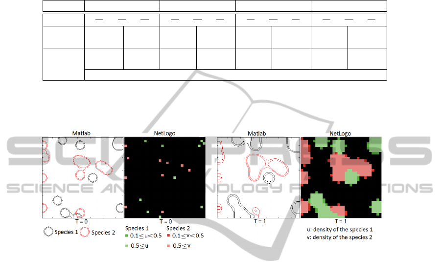
Fig. 1. Simulation with two species in case 2 with α
1
= α
2
= 1, β
1
= β
2
= 1, γ
1
= 1.5, γ
2
=
2.
Figure 1 stands for the diffusion of two species (green and red) with two program-
ming frameworks Matlab and NetLogo. With the NetLogo framework, bright color
presents the higher density than a threshold and the dark color presents the lower den-
sity than a threshold. With Matlab, the area inside the small circle presents the former,
the area inside the big circle and outside small circle presents to the latter. We can see
that two different programming frameworks give the same result.
As this model only represents the competition between to species, we have proposed
to generalize this case to a larger number of species.
2.2 Model of Nonlinear Diffusion of n Species with EDP
We expand the model to n species:
u
it
− ε
i
div
Q
k6=i
Φ (u
k
) ∇u
i
!
= u
i
α
i
−
P
n
j=1
β
ij
u
j
, (x, y) ∈ Ω, t > 0,
∇u
i
· n = 0 on δΩ × [0, +∞[,
u
i
(x, y, 0) = u
i0
(x, y) (x, y) ∈ Ω
(3)
22

The function Φ presents the influence of the diffusion of the other species in the
same area with the given species. This means that if the other species’s development
is too strong in the investigating area, the investigated species cannot diffuse (the case
whenΦ = 0). We consider the function of n species is equal to the composition of n
function of each species.
To better understand the behavior of this system of equations, we choose three levels
of species behavior: dominant, average and lower levels.
Fig. 2. Unequal competition between four
species: one dominant species, one average
species and two lower species.
Fig. 3. Equal competition between five average
species.
In the case of unequal competition (2), the dominant species grows faster than the
other species. In the case of equal competition (3), the species almost develop at the
same speed.
We also study the influence of inter-species and intra-species parameters on the spa-
tial distribution by calculating the average of the surface of each species. For example,
with five average species in case 2 of parameters α
i
, β
i
and γ
i
. We change the number
of initial points of each species. We run the program ten times and calculate the means
of them. Each time, the positions of the initial points of each species are selected at
random.
Fig. 4. The distribution of surfaces (number of patches) after averaging: Case (a): There are 5
initial points of each species. Case (b): There are 10 initial points of each species.
23

This figure represents the difference between the means of real surfaces and the
means of ideal surfaces of each species after ten times running the program. Case (a)
is the case in which there are five initial points of each species. Case (b) is the case
with ten initial points of each species. We can see that the distribution of surfaces is
dependent on the number of initial points.
2.3 Comparison between Isotropic Nonlinear Competition Model and
Anisotropic Competition Model with EDP
The previous model has been conceived to represent the competition between the plants
but the influence of the environment is not taken into account. We have thus proposed
the following models to consider the distribution of resources.
In the case of the nonlinear isotropic diffusion, the diffusion is isotropic but depends
on the gradient of resources. A resource function and a gradient of the resource function
are added in the diffusion term:
u
t
− ε
1
div (Φ (v) (Φ
1,s1
(R) + Φ
1,s2
(∇R∇u)) ∇u)
= u (α
1
− β
1
u − γ
1
v) , (x, y) ∈ Ω, t > 0,
v
t
− ε
2
div (Φ (u) (Φ
1,s1
(R) + Φ
1,s2
(∇R∇u)) ∇v)
= v (α
2
− β
2
v − γ
2
u) , (x, y) ∈ Ω, t > 0,
∇u · n = ∇v · n = 0 on δΩ × [0, +∞[,
u(x, y, 0) = u
0
(x, y), v(x, y, 0) = v
0
(x, y) (x, y) ∈ Ω
(4)
In the case of the anisotropic diffusion, a tensor is used to represent the direction of
resources:
u
t
− ε
1
div
Φ (v) Φ
2
(∇R∇u) ηη
T
∇u
+ div (Φ (v) Φ
1,s1
(R) ∇u)
= u (α
1
− β
1
u − γ
1
v) , (x, y) ∈ Ω, t > 0,
v
t
− ε
2
div
Φ (u) Φ
2
(∇R∇v) ηη
T
∇v
+ div (Φ (u) Φ
1,s1
(R) ∇v)
= v (α
2
− β
2
v − γ
2
u) , (x, y) ∈ Ω, t > 0,
∇u · n = ∇v · n = 0 on δΩ × [0, +∞[,
u(x, y, 0) = u
0
(x, y), v(x, y, 0) = v
0
(x, y) (x, y) ∈ Ω
(5)
where
Φ
1,s
∗
(x) =
h
∗
if thresoldM ax
∗
≤ x
h
∗
x
thresoldMax
∗
if thresoldM in
∗
≤ x < thresoldMax
∗
0 if x < thresoldM in
∗
s
∗
= (thresoldMax
∗
, thresoldM in
∗
, h
∗
)
Φ
2
(x) = Φ
1,s
∗
(x) with h
∗
= 1
−→
η =
−→
∇R
k∇Rk
24
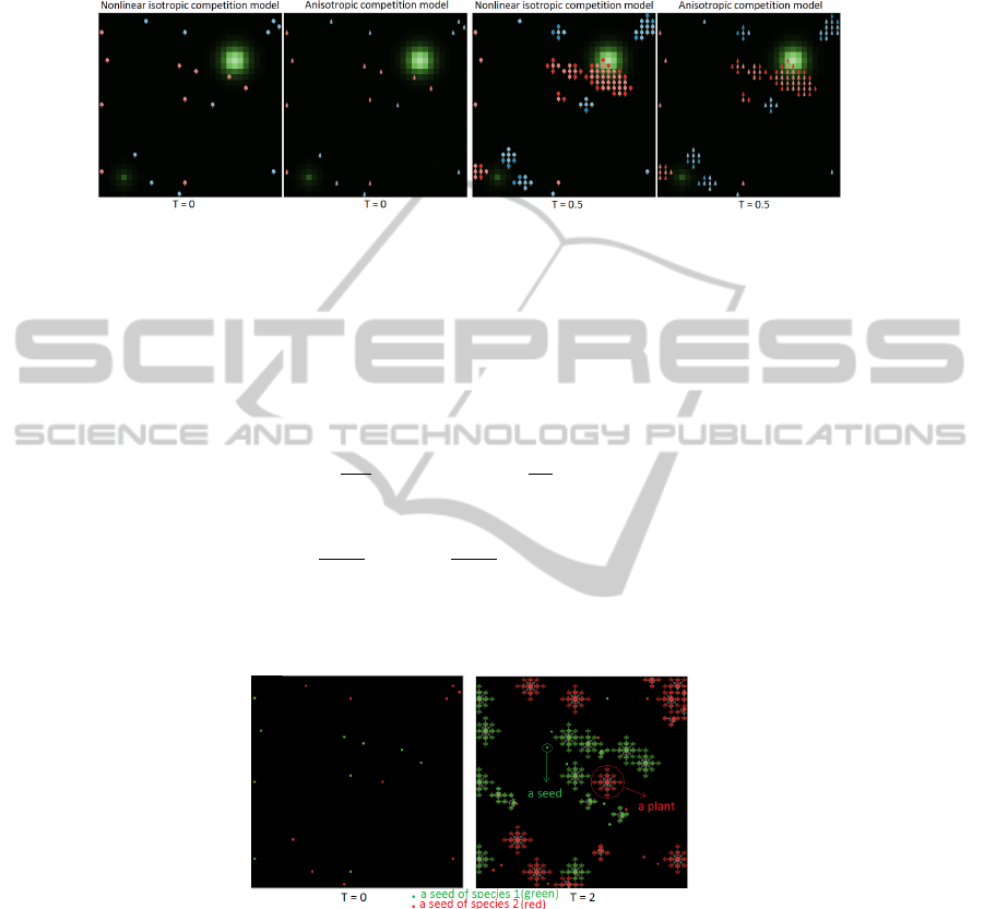
We present the results of the two approaches. The difference in the selected context
of resources is insignificant.
Fig. 5. The isotropic competition model and the anisotropic competition model.
2.4 Modeling Diffusion Species with MAS
In this model, we represent each individual in the community by an agent evolving on a
NxM grid of patches. As mentioned above, the diffusion of the population depends on 2
processes: the plants’ growth and their reproduction. The equation for the maintenance
and growth metabolism was given by [1]:
dm
dt
= am
3/4
1 −
m
M
1/4
(6)
where m is total body mass (m = m
c
N
c
); M is an asymptotic maximum body size,
asymptotic mass (M =
B
0
m
c
B
c
4
); a ≡
B
0
m
c
E
c
; B
0
is basic energy input; m
c
is mass of
a cell; E
c
is metabolic energy required to create a cell; B
c
is metabolic rate of a single
cell; N
c
is total number of cells. Practically, the spatial diffusion of the plant is then
proportional to its mass (see figure 6 - right).
Fig. 6. The development of 2 species with MAS.
Considering the reproduction of the species, we have taken inspiration from the Ne-
ture model [7] developed on the NetLogo framework to simulate a terrestrial ecosystem.
The model takes into account vegetal producers and their decomposers. Yet, it does not
consider the competition between the vegetal producers. Considering the competition
between producers and decomposers it is not symmetrical and we had to thus to propose
a specific model.
25

In our model, the intra-species and inter-species competitions are simply modeled
by the fact that only on plant at a time can be present on a given patch. When the
biomass of a plant exceeds the necessary threshold to become a mature plant, the plant
starts his reproduction. When a plant reaches its sexual maturity, it is considered that
a seed of the plant can be dropped according to a Poisson distribution (with parameter
λ = 50). The position where the seed falls is chosen randomly within a circle whose
center represents the father plant and the radius parameter (dist) is defined by the user
(see figure 6 - right). If the falling position is on an area outside the border or in an
area where there is another plant, the seed dies. We consider this corresponding to the
survivability of a seed in the wild.
Algorithm 1: Pseudocode of plant’s growth.
biomass = mass-of-seed;
while biomass ¡ maximum-biomass {
a =
B
0
∗m
c
E
c
;
delta-biomass =a ∗ mass
3/4
∗
1 −
mass
maximum-mass
1/4
;
biomass += delta-biomass;
}
Algorithm 2: Pseudocode of plant’s distribution.
if (biomass ¿= biomass-of-mature-plant and biomass ¡= maximum-biomass)
probability has a seed = Poisson distribution
if plant has a seed
position of seed is random within a circle with radius = dist until selected position is empty
2.5 Comparison between Model-based EDP and Model-based Agents
Figure 7 shows the comparison between the final state obtained with PDE and MAS
when the MAS model has different values of parameter “dist”. Parameter “dist” deter-
mines the distance between the position of the parent plant and the new seed. The closer
to the parent plant the new seeds are, the closer to the PDE the MAS model is.
To better understand the comparison between the two models, some key features
must be enlightened:
– The PDE model represents a global representation of the system. We can measure
the biomass on a given area (a patch) but we cannot know exactly how many indi-
viduals it corresponds to. This is a limitation of this model. In contrast, the MAS
model represents individuals. Yet, the MAS computation time may be very impor-
tant if the number of individuals and patches is high.
– In the MAS model, the spatial diffusion of a plant depends on 2 processes: the
growth and the reproduction of the plants. The growth factor is modeled by the
formula given in section 2.4. The reproduction depends on the maturity parameter,
the probability of producing a seed and the probability that a seed can survive.
Concerning the PDE model, the only parameter related to growth is α.
26
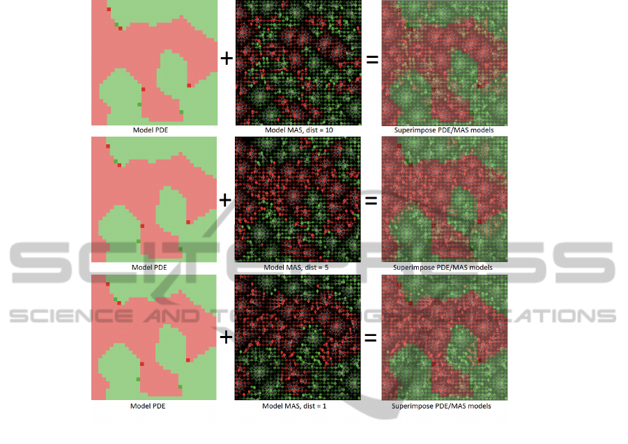
Fig. 7. The result of case 2 with model PDE, model MAS and the superimpose of two models.
– The rate of intra-species (β) and inter-species (γ) competition in the PDE model
corresponds respectively, in the MAS model, to the competitive behavior between
and individual and another individual of the same species and the competitive be-
havior between and individual and an individual of a different species. Yet, as in
the MAS model we do not make the difference between those two kinds of compe-
titions, it acts as if β = γ.
3 Conclusions
In this article, we have implemented [3]’s nonlinear diffusion of 2 species in competi-
tion. Besides, we have extended this model to a reaction-diffusion of one to n species in
which the competition between species happens but has no effect on the species’s living
environment. Moreover, we have also developed two diffusion models of two species in
which the diffusion of species is affected by environmental factors. In parallel, a sim-
ple MAS model was implemented in order to make the comparison with PDE model.
It would be interesting to evaluate how time is included in each model. Though basic
comparisons are made, they are to be discussed and studied so that we can combine
these two models and enjoy their advantages.
27

References
1. West, G. B., Brown, J. H., Enquist, B. J.: A general model for ontogenetic growth. Nature
413 (2001) 628–31
2. Bradley, L., Kilby, M., Call, R. E., Kopec, D., Capizzi, J., Langston, D., Claridge, J. D., Maloy,
O., DeGomez, T., Mikel, T., Doerge, T., Oebker, N., Green, J., Tipton, J., Gibson, R., Wilcox,
M., Gibson, R., Young, D., Grumbles, R.: Environmental factors that affect plant growth. In:
Arizona Master Gardener Manual. Arizona Cooperative Extension, College of Agriculture,
The University of Arizona, Arizona (1998) 30–33
3. El Hamidi, A., Garbey, M., Ali, N.: On nonlinear coupled diffusions in competition systems.
Nonlinear Analysis: Real World Applications 13 (2011) 1306–1318
4. Cosner, C., Lazer, A. C.: Stable Coexistence States in the Volterra-Lotka Competition Model
with Diffusion. SIAM 44 (1984) 1112–1132
5. Hsu, S.b., Waltman, P.: On a System of Reaction-Diffusion Equations Arising From Compe-
tition in an Unstirred Chemostat. SIAM 53 (1993) 1026–1044
6. Karami, F.: Limite singuli
`
ere de quelques probl
`
emes de R
´
eaction Diffusion : Analyse
math
´
ematique et num
´
erique. PhD thesis, Picardie Jules Verne (2007)
7. Grueters, U.: Neture - a NetLogo model that simulates how Nature works. (2011)
8. Treuil, J. P., Drogoul, A., Zucker, J. D.: Mod
´
elisation et simulation
`
a base d’agents: exemples
commentes outils informatiques et questions th
´
eorique. (2008)
28
