
Phase-differencing in Stereo Vision
Solving the Localisation Problem
J. M. H. du Buf, K. Terzic and J. M. F. Rodrigues
Vision Laboratory, LARSyS, University of the Algarve, 8005-139 Faro, Portugal
Keywords:
Complex Gabor Filters, Phase, Disparity, Lines, Edges, Localisation.
Abstract:
Complex Gabor filters with phases in quadrature are often used to model even- and odd-symmetric simple
cells in the primary visual cortex. In stereo vision, the phase difference between the responses of the left and
right views can be used to construct a disparity or depth map. Various constraints can be applied in order to
construct smooth maps, but this leads to very imprecise depth transitions. In this theoretical paper we show, by
using lines and edges as image primitives, the origin of the localisation problem. We also argue that disparity
should be attributed to lines and edges, rather than trying to construct a 3D surface map in cortical area V1. We
derive allowable translation ranges which yield correct disparity estimates, both for left-view centered vision
and for cyclopean vision.
1 INTRODUCTION
Unquestionably, the phase of Gabor filters provides
useful information for stereo disparity. It is also bi-
ologically plausible, because simple cells in the pri-
mary visual cortex (area V1) are often modelled by
complex Gabor filters with phases in quadrature. The
cortical structure in hypercolumns brings information
of the left and right eyes closely together, suggesting
that stereo processing already starts in area V1.
Since the seminal work of Sanger (1988) and
Jenkin and Jepson (1988) exactly 25 years ago, the
phase model has attracted a lot of attention. Being
a very intuitive and appealing model, its simplicity
seemingly contradicts that lot of attention. Indeed,
results obtained with real images, also with random
dot stereograms, are not very good, and one might
say that the model appears to be a blessing, but a
cursed one. Most researchers may be aware of the
model’s sting, but seem to have problems in locat-
ing and characterising that sting. Part of the prob-
lem may be due to exaggerated expectations: a very
simple model which should satisfy two conflicting
requirements, namely to provide a reconstruction of
smooth and continuous surfaces, yet in combination
with sharp and precisely located depth transitions.
In this theoretical paper we will therefore focus on
the localisation problem of the simple phase model.
For an overview of alternative biological disparity
models see (Read and Cumming, 2007). In the next
two sections we present a brief overview of earlier
work, including Sanger’s, to illustrate the “sting,” the
constraints which have been and still are applied in
estimating disparity, and some important assumptions
which should be taken into account. Section 4 deals
with the simplest case, namely positive lines. Neg-
ative lines and edges are analysed in Section 5. In
Section 6 we analyse two combinations: line clusters
and bars. In Section 7 we present a summary of the
phase model and a way to circumvent the problems.
How local phase should be used in one-sided views
is described in Section 8, whereas cyclopean vision is
described in Section 9. An alternative phase model
which is based on complex conjugate responses is
analysed in Section 10. We conclude with a small
discussion in Section 11.
2 MANY CONSTRAINTS AND
YET POOR RESULTS
Like others, Sanger may have realised the localisa-
tion problem, but he focused on random dot stere-
ograms (RDSs). He introduced a set of constraints
together with a smoothing step in order to obtain
model predictions which, at least, resemble perceived
disparity of the RDSs. First, Gabor filter responses
are thresholded such that those with insufficient am-
plitude and therefore meaningless phase are ignored.
254
M. H. du Buf J., Terzic K. and M. F. Rodrigues J..
Phase-differencing in Stereo Vision - Solving the Localisation Problem.
DOI: 10.5220/0004349702540263
In Proceedings of the International Conference on Bio-inspired Systems and Signal Processing (BIOSIGNALS-2013), pages 254-263
ISBN: 978-989-8565-36-5
Copyright
c
2013 SCITEPRESS (Science and Technology Publications, Lda.)

Second, a confidence is computed using responses of
the left and right views, with similar responses yield-
ing a higher confidence, and the disparity estimates
obtained at multiple filter scales are averaged by us-
ing the confidences. This is supposed to suppress
disparity estimates distorted by noise in each filter’s
frequency band as well as those beyond the detection
limit of each filter. The above criteria are all merely
based on amplitudes, not on any phase or disparity in-
formation. Third, a second-level confidence is used
to exclude scales with disparity estimates which de-
viate from the (weighted) average, i.e., outliers, now
taking into account both the amplitudes and disparity
estimates at all applied scales. Finally, the second-
level confidence is used to create a smooth surface,
assuming that nearby points should have similar dis-
parities. This is a nonlinear spatial filtering because
of the weighting of neighbouring disparity values by
their confidences. Despite all processing before and
after computing the phase differences, with emphasis
on image noise, detection limits and local consistency
of disparity estimates, Sanger’s results are extremely
noisy and imprecise in terms of localisation; see also
(Jenkin and Jepson, 1988).
The same observation holds when looking at more
recent results. For example, Fr
¨
ohlinghaus and Buh-
mann (1996) considered disparity estimation an ill-
posed problem which requires regularisation in order
to produce smooth results, and thereby lose, not to
say sacrifice, good localisation. This effect is clearly
visible in most if not all results which employ real im-
ages (Pauwels et al., 2012). Solari et al. (2001) pre-
sented an alternative phase-differencing model (see
Section 10), perhaps more in line with biological pro-
cessing, but without any postprocessing or regularisa-
tion. Their results are also very noisy, and neat ver-
tical edges look crooked, as if they were distorted by
some “random zig-zag filter.”
Hence, one cannot deny that there must be some
obscure problem lurking in phase differencing and, to
the best of our knowledge, this “sting” has not yet
been clearly identified. One of the most profound and
recent analyses, by Monaco et al. (2008), addresses
applicable constraints, but assumes as principal im-
age model white noise, like in RDSs. The main con-
straints, as already formulated and applied in earlier
work (Sanger, 1988; Fleet and Jepson, 1990; Fleet
et al., 1991), serve to avoid regions where the instan-
taneous frequency (the derivative of the phase signal)
deviates too much from the filter’s central frequency,
like at phase jumps caused by phase wrapping of the
arctangent function, and to avoid singularities where
the real and imaginary response components are zero
and the phase is not defined. As we will see below,
such constraints are not really beneficial, not to say
completely useless, in the case of real images domi-
nated by lines, bars and edges.
3 A VERY SIMPLE MODEL IN A
VERY COMPLEX SYSTEM
In contrast to other approaches we will ignore RDSs
and the white noise image model. Simple and com-
plex cells in area V1 may code noise patterns, such as
stochastic textures, but their main purpose is to code
lines and edges for object recognition and brightness
perception (Rodrigues and du Buf, 2009). When fo-
cusing on models for disparity, one easily forgets that
there also are other cells for coding specific patterns,
like individual bars and periodic gratings (du Buf,
2007) and dot patterns like the ones used in Sanger’s
RDSs (Kruizinga and Petkov, 2000). Our insight into
the complexity of the visual system, with a myriad of
different cell functions and a zillion of connexions, is
still rather poor. It may make sense to develop mod-
els for specific purposes, like one model for RDSs and
another one for lines and edges, before trying to de-
velop a unified model.
We explicitly question the requirement that, at a
very low level in the visual system such as in areas V1
and V2 etc., our visual system reconstructs a “replica”
of our 3D environment. The idea of attributing dis-
parity information to planar and curved surfaces may
seem to make sense. It is the same idea as that be-
hind brightness perception of surfaces: a realistic and
precise reconstruction of scenes and objects, like a
photograph, every pixel of the photograph even com-
plemented by depth information. But philosophically
that idea has a big problem. If 3D scenes are recon-
structed at an early stage in vision, then there should
be another, virtual observer in our brain who analyses
that reconstruction. If that other observer also recon-
structs, there should be yet another one. Hence, this
reasoning leads to infinite regress.
Taking into account that the visual system applies
hierarchical processing, from simple elementary fea-
tures to increasingly more complex ones, from syn-
tax to semantics, the only solution is to work with
features. Like in brightness perception, where lo-
cal brightness is only attributed to lines and edges in
a multi-scale representation (Rodrigues and du Buf,
2009), the same can be done with disparity. Since
many simple and complex cells in V1 (and other cells
in higher areas) are disparity tuned, and since those
cells provide an efficient vehicle for line and edge
coding, disparity can be attibuted to detected lines and
edges. This yields a sort of wireframe representation
Phase-differencinginStereoVision-SolvingtheLocalisationProblem
255
-3
-2
-1
1
2
3
-1.0
-0.5
0.5
1.0
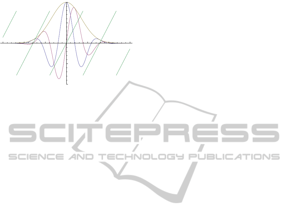
Figure 1: The example simple cells: real (cosine) and
imaginary (sine) responses, the Gaussian envelope, and the
wrapped phase divided by ω
0
= 4. Note: π/4 ≈ 0.8.
as used in computer graphics. Such a wireframe rep-
resents structural shape properties of objects, includ-
ing existing patterns on their surfaces. The big advan-
tage is that there is no localisation problem: if a line or
edge is detected in the left view, the response (phase)
in the right view at exactly the detected position can
be employed. In other words, the localisation prob-
lem is reduced to a detection problem (Rodrigues and
du Buf, 2009). Below we illustrate the localisation
problem, and we show how phase information should
be exploited.
4 THE POSITIVE LINE CASE
As usual, a complex Gabor function which is used to
model simple and complex cells in V1 is defined by
G(x) = e
−x
2
/2σ
2
+iω
0
x
= e
−x
2
/2σ
2
(cosω
0
x +i sin ω
0
x).
(1)
Below we will illustrate results using specific val-
ues: 2σ
2
= 1 and ω
0
= 4. The latter yields a pe-
riod T
0
= 1/F
0
= 2π/ω
0
= π/2 ≈ 1.6. An input sig-
nal defined on x is convolved with G(x), after which
we can compute the real (Re) and imaginary (Im) re-
sponses of the even- and odd-symmetric simple cells.
The amplitude (Mod) is (Re
2
+ Im
2
)
1/2
as a model of
complex cells, and finally the phase θ is the argument
(Arg) of the complex response. See Fig. 1.
The simplest case to study is one Dirac function
with “amplitude” 1 at x = 0. Because of its sift-
ing property, the response equals Eq. 1. The phase
model yields θ(x) = ω
0
x, which comprises the filter’s
frequency ω
0
. There are two possibilities to elimi-
nate this frequency component from θ: (a) divide by
ω
0
, which implicitly assumes that some cells know
this parameter, or (b) divide by the instantaneous fre-
quency
¯
ω(x) =
˙
θ(x), the derivative of θ(x). The use of
the instantaneous frequency assumes that the cells do
not have access to the value of parameter ω
0
, but it re-
quires an additional cell layer which implements the
derivative operator. In this trivial case
˙
θ = ω
0
, such
that θ/
˙
θ = x. This means that the phase is an ideal ve-
hicle for translation estimation, both for disparity and
optic flow (Fleet and Jepson, 1990; Fleet et al., 1991).
The above analytic analysis yields a perfect result
for translation estimation, even on [−∞,∞] and for ar-
bitrary values of σ and ω
0
, but there is a big prob-
lem: ArgG(x) requires the arctan operator, such that
the phase is limited to (−π,π], it is wrapped around,
and it is periodic. Hence, only valid is |ω
0
x| ≤ π such
that θ/
˙
θ = x for |x| < π/ω
0
= T
0
/2, i.e., on exactly
one period of G(x). In the last formula we wrote <
instead of ≤ because of the derivative operator, which
must avoid the two phase jumps of 2π, but this is of
secondary importance.
The simplest case of disparity estimation involves
one positive Dirac seen against a homogeneous back-
ground. We will focus on near disparity: a thin, white
pole, for example that of a traffic sign, seen against
a dark wall. Now we introduce left (L) and right (R)
views with a shift of ±δ relative to x = 0. Near dis-
parity implies that in the left view the Dirac shifts to
the right and in the right view it shifts to the left. The
goal is to estimate the total shift of 2δ.
We have L(x) = G(x − δ) and R(x) = G(x + δ),
therefore θ
R
(x) = ω
0
(x + δ), θ
L
(x) = ω
0
(x − δ), and
let us define disparity as is usually done by D(x) =
∆θ/
˙
θ, where ∆θ = θ
R
− θ
L
. In this simple case we
can divide ∆θ by ω
0
. Anyhow, the result is 2δ. This
analytic solution is correct: it is the left-sided view in
which the right-sided projection is shifted 2δ to the
right. However, D(x) = 2δ holds for −∞ < x < ∞ be-
cause we are working with ideal and generalized func-
tions. In practice we can limit the interval by thresh-
olding the modulus (the responses of complex cells:
the Gaussian envelopes of the Gabor filters), but only
the maximum is well defined. Furthermore, the arc-
tan operator must be applied, to both L and R. As a
result, both θ
L
and θ
R
are restricted to ±π. Normally,
two constraints are applied (Monaco et al., 2008): if
¯
ω =
˙
θ, then |
¯
ω − ω
0
| < ρ, which serves to stay away
from the phase discontinuities where the phase wraps
around, also to avoid strong phase nonlinearities (see
below), but here this is useless because
¯
ω = ω
0
, ex-
cept at the phase jumps. The second constraint serves
to avoid singularities where both real and imaginary
responses are zero, which is also useless here.
What are the problems introduced by the arctan
function? The two phases are linear and zero at
the positions of the two Diracs, i.e., they are paral-
lel and shifted functions. This means that there are
BIOSIGNALS2013-InternationalConferenceonBio-inspiredSystemsandSignalProcessing
256

two crossings at +π and two at −π, and we need to
take the inner two for the validity range of ∆θ: this
yields δ − π/ω
0
< x < −δ + π/ω
0
, or δ − T
0
/2 < x <
−δ + T
0
/2. But we do not know δ, we only obtain
D(x). A first conclusion is that the localisation of the
Dirac is lost: D(x) = 2δ for δ−T
0
/2 < x < −δ+T
0
/2.
Beyond these two limits, the phases are wrapped and
D(x) becomes negative: D(x) = 2δ − T
0
. And D(x)
is periodic (T
0
). If δ = T
0
/2, perfect localisation is
obtained (2δ only in x = 0), but this is flanked by neg-
ative values over the entire period. If δ increases, or
ω
0
decreases, the value of D(x ≈ 0) even becomes
negative! One can easily see that for 2δ → 0 almost
the entire period T
0
is correct (D = 2δ) but localisa-
tion is completely lost. Therefore, a second conclu-
sion is that the disparity estimates may be correct on
some intervals, but wrong (negative) on the remain-
ing intervals. And these intervals are a function of
scale, i.e., of ω
0
relative to the real disparity. If multi-
ple scales are applied, the problem can only be solved
by combining the various results, like Sanger did, but,
given his noisy results, this is not an easy problem. As
we will see in the next section, the confusion is even
much worse.
5 NEGATIVE LINES AND EDGES
A dark line against a homogeneous background, for
example a thin black pole in front of a white or gray
wall, is of course modelled by a negative Dirac func-
tion, and intuitively one expects results similar to a
positive Dirac but with negated responses. Indeed, we
obtain the following response:
F(x) = −G(x) = e
−x
2
/2σ
2
+i(ω
0
x+π)
= e
−x
2
/2σ
2
(−cosω
0
x − i sin ω
0
x). (2)
The phase is θ(x) = ω
0
x + π, which means that in
practice there is a phase discontinuity exactly at the
line’s position. Therefore, translation estimation is
not similar to that in case of a positive Dirac: (1) at
x = 0 the phase is undefined or may switch randomly
between π and −π because of noise; (2) for x > 0 the
relative translation is −π+ω
0
x, so one could add π to
correct this; (3) for x < 0 it is π + ω
0
x and one could
subtract π.
In the case of disparity (two shifted, negative
Diracs) we have θ
R
= ω
0
(x + δ) + π and θ
L
= ω
0
(x −
δ) + π, such that ∆θ = 2δω
0
, but this is the analyt-
ical solution for x ∈ [−∞,∞]. The difference of the
wrapped phases is negative around x = 0 for small δ
due to the two discontinuities at x = ±δ. To be pre-
cise, for δ < π/ω
0
= T
0
/2 the disparity estimate at
-3
-2
-1
1
2
3
-1.0
-0.5
0.5
1.0
Figure 2: Phase plots (divided by ω
0
= 4) of responses to
positive and negative lines and edges at x = 0. Crossing the
vertical axis at x = 0 are, from top to bottom: L
−
, E
−
, L
+
,
E
+
and L
−
.
x = 0 is 2δ − 4π/ω
0
= 2δ − 2T
0
because of the two
phase jumps of 2π, and for δ > T
0
/2 it is 2δ − T
0
. In
other words, at δ = T
0
/2 the disparity estimate jumps
from one wrong value to another wrong value. The
phase constraint |
¯
ω − ω
0
| < ρ can be used to skip the
phase discontinuities, but these are only a few points
on x and all other disparity estimates on x are com-
pletely useless.
Edges are much more complicated to deal with an-
alytically, because responses of complex Gabor filters
are complex error functions. Fortunately, it has been
shown that complex error functions can be well ap-
proximated by Gabor functions, by tweaking the two
parameters a little bit (du Buf, 1993). He called this
an abnormal scaling of the Gabor function. If a nor-
mal scaling is obtained by σs and ω
0
/s, with s the
scale parameter, an abnormal scaling, i.e., approxi-
mation of the error function which is the response of
a normally scaled Gabor filter, is obtained by
¯
σ = σ/a
and
¯
ω
0
= ω
0
/b, where σ and ω
0
are the parameters of
the Gabor filter. Below we apply this approximation
and deal with edge responses through Gabor func-
tions. We will not include the proportionality con-
stant of the error function, because this appears in the
modulus of the Gabor response and it simply disap-
pears in the phase. For the sake of simplicity we even
write σ and ω
0
in stead of
¯
σ and
¯
ω
0
(please recall that
the instantaneous frequency must be used, which is
approximately
¯
ω
0
).
Going from left to right, a positive edge E
+
is de-
fined as a positive transition in x = 0: a step with value
−1 for x < 0 and +1 for x > 0. Similarly, a negative
edge is defined by E
−
= −E
+
. The response to a pos-
itive edge is described by
F(x) = G
+
(x) = e
−x
2
/2σ
2
+i(ω
0
x−π/2)
= e
−x
2
/2σ
2
(sinω
0
x − i cos ω
0
x). (3)
Phase-differencinginStereoVision-SolvingtheLocalisationProblem
257

The phase is ω
0
x − π/2, i.e., in x = 0 it is −π/2
(we note that this is different from the value π/2 ob-
tained by du Buf (1993), because he used correlation
whereas here we use convolution). Similarly, the re-
sponse to a negative edge is described by
F(x) = G
−
(x) = e
−x
2
/2σ
2
+i(ω
0
x+π/2)
= e
−x
2
/2σ
2
(−sinω
0
x + i cos ω
0
x). (4)
The phase is ω
0
x + π/2, i.e., in x = 0 it is π/2. The
phase values at the edges imply that the pivot points
through which the linear phase plots rotate as a func-
tion of the scale (ω
0
) are at x = 0 and θ = ±π/2, with
the usual discontinuities at ±π. Figure 2 summarises
the different phase behaviours of positive and nega-
tive lines and edges at position x = 0.
Suppose that there is only one positive edge in a
neighbourhood with a L-R shift of 2δ. We therefore
have
L(x) = G
+
(x − δ) = e
−(x−δ)
2
/2σ
2
+i(ω
0
(x−δ)−π/2)
. (5)
The phase is θ
L
= ω
0
(x − δ) − π/2. We also have
R(x) = G
+
(x + δ) = e
−(x+δ)
2
/2σ
2
+i(ω
0
(x+δ)−π/2)
(6)
with a phase θ
R
= ω
0
(x + δ) − π/2, such that ∆θ =
θ
R
− θ
L
= 2ω
0
δ and
˙
θ
L
=
˙
θ
R
= ω
0
. However, phase
wrapping implies that ∆θ may be negative around x =
−δ and positive around x = δ, obviously with a dis-
continuity in between, and this discontinuity shifts as
a function of the scale (ω
0
). For example, if δ = T
0
/4,
the discontinuity will be exactly at x = 0. To the right,
the phase difference is correct (ω
0
2δ) until θ
R
reaches
π, i.e., for 0 < x < T
0
/2. To the left, the phase differ-
ence is wrong (ω
0
2δ − 2π) because θ
L
wraps around
at x = 0. This phase jump of 2π in combination with
∆θ = θ
R
−θ
L
divided by ω
0
yields the wrong disparity
2δ−T
0
. The wrong phase difference and disparity are
obtained until θ
R
reaches −π, i.e., for −T
0
/2 < x < 0.
Hence, one half of the period is correct and the other
half is wrong, this is repeated periodically (T
0
), and
there is absolutely no localisation except if we trun-
cate the result somehow using the modulus (responses
of complex cells). Disparity estimation in the case of
one negative edge is similar, yet with the same prob-
lems.
6 LINE CLUSTERS AND BARS
If lines and edges are well separated, they can be
detected individually because the modulus will show
distinct maxima and their phases will not be distorted
by interference effects (du Buf, 1993). The question
is what happens when they are closer together, form-
ing clusters of lines and bars. We first analyse line
clusters and then bars.
There are many possibilities concerning distances
and amplitudes. For the sake of simplicity let us take
three equidistant lines (Diracs) with “amplitude” 1
and centered around x = 0:
F(x) = G(x) + G(x + δ) + G(x − δ). (7)
What is the influence of the Diracs at x = ±δ on the
response of the Dirac at x = 0? The exact solution is
F(x) = G(x) · [1 + 2e
−δ
2
/2σ
2
cos(ω
0
δ + i
2xδ
2σ
2
)], (8)
where
2cos(ω
0
δ + i
2xδ
2σ
2
) = e
−2xδ/2σ
2
+iω
0
δ
+ e
2xδ/2σ
2
−iω
0
δ
.
(9)
Using a Taylor series around x = 0 (or e
z
≈ 1 + z) re-
sults in
F(x)/G(x) = 1 + 2e
−δ
2
/2σ
2
(cosω
0
δ − i
xδ
σ
2
sinω
0
δ).
(10)
In order not to influence the phase of the response of
G(x) around x = 0, i.e., ω
0
x, this function must be
real. We see that there are two possibilities. One is
δ σ
2
, which relates the distance to the width of
the envelope. The other is sinω
0
δ = 0. This means
ω
0
δ = kπ, or δ = kπ/ω
0
= kT
0
/2. There are only two
possibilities in practice: 0 and π/ω
0
. When δ = 0, (8)
results in F(x) = 3G(x), as expected: three Diracs in
x = 0. When δ = π/ω
0
= T
0
/2, (8) results in
F(x)/G(x) = 1 − e
π/σ
2
ω
0
(e
−x
+ e
x
)e
−π
2
/σ
2
ω
2
0
, (11)
which is also real. In contrast to these two cases, we
can expect the biggest problem (worst case?) when
in (10) the imaginary part is maximum: sin ω
0
δ = 1
or δ = π/2ω
0
= T
0
/4. Substituting this δ in (8) and
approximating exp(−x)− exp(x) by −2x gives
F(x)/G(x) = 1 − ix2e
π/2σ
2
ω
0
−π
2
/8σ
2
ω
2
0
= 1 − ixA.
(12)
The modulus is (1 + x
2
A
2
)
1/2
and the phase is
−arctan(xA). With arctan(xA) ≈ xA for |xA| ≤ 1, i.e.,
x ≈ 0, we then obtain
F(x) = e
−x
2
/2σ
2
p
1 + x
2
A
2
e
i(ω
0
x−Ax)
. (13)
When dividing θ(x) = (ω
0
− A)x by ω
0
, translation
estimation gives θ(x)/ω
0
= (ω
0
− A)x/ω
0
= x(1 −
A/ω
0
). Substitution of the values of σ and ω
0
gives
A = 3.76, A/ω
0
= 0.94, and x(1 − A/ω
0
) = 0.06x.
Obviously, this is not correct, and wrong translation
estimation will result in wrong disparity estimation.
When using the instantaneous frequency instead, we
BIOSIGNALS2013-InternationalConferenceonBio-inspiredSystemsandSignalProcessing
258

divide θ(x) = (ω
0
− A)x by
˙
θ(x) = ω
0
− A and obtain
θ/
˙
θ = x, which is the correct translation estimation.
However, we forgot several approximations like |x| ≈
0 and |xA| ≤ 1. The latter means |x| ≤ 1/A ≈ 0.25,
which is of the order of T
0
/6. Hence, at and beyond
T
0
/6 the analytical result is not reliable. Please recall
that we analysed the case δ = T
0
/4. Hence, we saw
that the instantaneous frequency must really be used
and we can expect that a small cluster of close lines
may behave as one line.
Concerning bars, a positive bar with amplitude 1,
centered at x = 0 and with width 2δ, is defined by
B
+
(x) = 0.5{E
+
(x + δ) + E
−
(x − δ)}. If δ is very
small, we expect responses similar to those of lines
(Diracs), but because there are two edges the analysis
is more complicated. Using the edge responses de-
fined before, we obtain
R(x) =
1
2
{G
+
(x + δ) + G
−
(x − δ)}
=
1
2
{e
−(x+δ)
2
/2σ
2
(−ie
iω
0
(x+δ)
)
+e
−(x−δ)
2
/2σ
2
(ie
iω
0
(x−δ)
)}. (14)
In order to see what this means, we can first look at
the response in the centre:
R(0) =
1
2
e
−δ
2
/2σ
2
{−ie
iω
0
δ
+ ie
−iω
0
δ
}
= sinω
0
δ · e
−δ
2
/2σ
2
. (15)
This is real and we can distinguish the following cases
based on the sine function (please recall that the width
is 2δ and that the period of the Gabor function is T
0
=
2π/ω
0
):
• For δ = 0 there is a singularity in x = 0 because
both the real and imaginary responses are zero.
One could take the limit δ → 0 to approximate the
Dirac case, but the width approaches 0 whereas
the bar’s amplitude remains 1.
• If 0 < ω
0
δ < π, i.e., 2δ < T
0
, the phase is zero in
x = 0, which corresponds to that of a positive line.
Here we can have a relatively narrow bar which
behaves as a line, but also a broad one because
0 < 2δ < T
0
, i.e., a width up to one period. In
the case of a broad bar, the two edges could be
detected separately.
• For ω
0
δ = π (2δ = T
0
) there is again a singularity
at x = 0.
• For π < ω
0
δ < 2π the phase in x = 0 is ±π, which
indicates a negative line, but this occurs for T
0
<
2δ < 2T
0
where the individual edges are detected
and the modulus in x = 0 is small.
This was the response in the centre, so now we can
analyse the responses at the edge positions. If we
-3
-2
-1
1
2
3
-1.0
-0.5
0.5
1.0
Figure 3: Phase plots of three lines at positions -0.1, 0 and
0.1 and bars with edges at -0.1 and 0.1. A cluster of three
close positive lines and a narrow positive bar behave as one
positive line (phase through the origin). The negative ver-
sions behave as one negative line (the phase crosses the ver-
tical axis at ±0.8). Note: π/4 ≈ 0.8.
choose as example ω
0
δ = π/2 or 2δ = T
0
/2 (see the
second case above), it follows from (14) that
R(−δ) = −
1
2
i(1 + e
−2δ
2
/σ
2
). (16)
Hence, R(−δ) ≈ −i if δ
2
σ
2
(the phase is −π/2).
Similarly, we obtain R(δ) ≈ i (the phase at the other
edge is π/2). Since the response R(0) is real, the
phase can be approximated by θ(x) ≈ (x/δ)(π/2) =
ω
0
x inside the bar. Outside the bar, the response and
therefore the phase is dominated by the positive edge
on the left side, and by the negative edge on the right
side, both with a component ω
0
x (because of the ap-
proximation of the complex error function this is
¯
ω
0
x)
and with a phase of ±π/2 at the two edges.
Figure 3 shows that a cluster of close lines and a
narrow bar indeed behave as a line, both in the posi-
tive and negative cases. Because we divided the phase
by ω
0
in stead of the instantaneous frequency, the
slopes are slightly different.
7 STINGS AND TWEEZERS
From the above analyses we may conclude that the
simple phase model is not really simple. There are se-
rious problems involved in obtaining reliable dispar-
ity estimates, and these can explain the poor results
which have been obtained in previous work (Sanger,
1988; Jenkin and Jepson, 1988; Fr
¨
ohlinghaus and
Buhmann, 1996; Solari et al., 2001; Pauwels et al.,
2012). And instead of one “sting” of the model we
have identified three stings: (1) phases and phase dif-
ferences are not localised, which may be an advan-
tage when creating a smooth depth map but it comes
at the cost of sacrificing any neat depth transitions;
Phase-differencinginStereoVision-SolvingtheLocalisationProblem
259

-1.5
-1.0
-0.5
0.5
1.0
1.5
-1.0
-0.5
0.5
1.0
Figure 4: Plots of ∆θ/ω
0
in the case of δ = T
0
/4 ≈ 0.4,
hence a real disparity of 0.8. In this case half the period
is correct (at top) and the other half is wrong (at bottom).
In order to avoid clutter, the disparities of a negative line,
positive edge and negative edge are shifted higher 0.1, 0.2
and 0.3, respectively, relative to that of a positive line. If
δ increases, the intervals with the correct disparity (at top)
become smaller, those with wrong disparity (at bottom) be-
come larger.
(2) phase differences may be correct on some inter-
vals of the filter’s period, but they are wrong on the
remaining intervals, and these intervals are repeated
periodically; and (3) the intervals with correct and
wrong phase differences depend on the wavelengths
of the filters in relation to the real disparity, but also
on the local image structure, where negative lines are
even disastrous. In other words, the phase differ-
ence may be easy to compute but yields totally con-
fusing and even contradictory results. Figure 4 sum-
marises the confusion. If a fronto-parallel planar sur-
face with a certain disparity is decorated with peri-
odic and well separated positive and negative lines
and edges, disparity estimation is doomed to produce
a randomly corrugated surface. In random dot stere-
ograms (Sanger, 1988; Jenkin and Jepson, 1988) and
in white noise stereograms (Monaco et al., 2008; So-
lari et al., 2001) there are always local fluctuations
which cause random phases, so how can one expect
to obtain e.g. flat surfaces? It seems that all process-
ing applied targets smooth surfaces. Even more ad-
vanced processing schemes, in which disparity esti-
mation starts at a coarse scale and is refined at pro-
gressively finer scales, seem to target only smooth
surfaces such that well-defined depth transitions at
high-contrast object boundaries often produce disas-
trous results (Pauwels et al., 2012).
Focusing on low-level processing, also a solu-
tion became obvious for tweezing the stings from the
model: the only way to obtain reliable and precise dis-
parity information is to check the local image struc-
ture, i.e., to detect lines and edges and to attribute dis-
parity only to detected events. Therefore one solution
is to combine the phase with line and edge detection:
we detect a line or an edge at a certain position in L,
and take the phase in R at the same position. We will
see that we need to detect the same event type in L
and R in order to avoid problems. One might say that
we therefore apply feature matching: a positive edge
in R must match a positive edge in L, hence the spa-
tial distance is available and therefore explicitly the
disparity. However, we assume that the cells in the
retinotopic mapping do not have access to their ab-
solute position. We only assume that there are cell
clusters in the direction of the simple cells and in a
certain neighbourhood with a size related to the scale
(and event type; see below). This is explained in the
following section. The next section deals with cyclo-
pean vision.
8 USING THE PHASE OF ONE
VIEW
In what follows we assume that the system detects
events in L and analyses R for making sure that there
is no other near event which destroys the correct phase
information. Now, assume that event detection in L
and R works, i.e., there is a good detection model. As
before, we assume near disparity of 2δ with a right-
shift of δ in L and a left-shift of δ in R. Hence, events
are detected in L at x = δ. In R we have
R(x) = e
−(x+δ)
2
/2σ
2
+i(ω
0
(x+δ)+φ
0
)
(17)
and, similarly, in L we have
L(x) = e
−(x−δ)
2
/2σ
2
+i(ω
0
(x−δ)+φ
0
)
(18)
with phases θ
R
= ω
0
(x+δ)+φ
0
and θ
L
= ω
0
(x−δ)+
φ
0
. The constant phase component φ
0
is 0 for a posi-
tive line (L
+
), ±π for a negative line (L
−
), −π/2 for a
positive edge (E
+
), and π/2 for a negative edge (E
−
).
In all four cases we substitute x = δ in both L(x) and
R(x) and obtain a disparity ∆θ/
˙
θ = 2δ in x = δ be-
cause
˙
θ =
˙
θ
L
=
˙
θ
R
= (
˙
θ
R
+
˙
θ
L
)/2 = ω
0
.
What are the constraints? Because there are no
singularities in case of isolated events, we can re-
strict the analysis to phase discontinuities, normally
expressed by the constraint |
˙
θ − ω
0
| < ρ. In our case,
where we detect events in L with specific phase val-
ues, there are no phase jumps at event positions (only
negative lines must be treated carefully) and we must
only avoid phase jumps in R. If we increase δ starting
with a small value, the phase difference increases lin-
early until θ
R
reaches π, where it wraps around to −π,
and then increases again linearly. Hence, the above
constraint only serves to avoid the phase jump, but
not the region beyond it. If the primary phase region
BIOSIGNALS2013-InternationalConferenceonBio-inspiredSystemsandSignalProcessing
260

is the one before the first phase jump, then which pri-
mary regions yield a valid phase difference? If we
make phase plots with the different values of φ
0
, we
can easily see that the translation before θ
R
reaches π
is largest for a negative line and smallest for a nega-
tive edge. The specific ranges are: 2δ
L
+
< (1/2)T
0
,
2δ
L
−
< T
0
, 2δ
E
+
< (3/4)T
0
, and 2δ
E
−
< (1/4)T
0
.
Please recall that in case of edges we should have
written
¯
T
0
because of
¯
ω
0
which results from approxi-
mating the complex error function responses by com-
plex Gabor functions, and this is obtained by comput-
ing the instantaneous frequency
˙
θ ≈
¯
ω
0
.
Hence, there are four different valid intervals for
the four event types. Beyond these intervals, i.e., for
larger disparities, in all four cases we get 2δ − T
0
be-
cause of the phase jump of −2π, which, divided by
˙
θ
or ω
0
, results in −T
0
. This phase difference is neg-
ative and therefore completely wrong. Although the
constraint |
˙
θ − ω
0
| < ρ may be met at all positions
except at the phase jump, which can be skipped, this
is not sufficient because both (1) the phase jump in R
must be skipped and (2) the region with the negative
disparity estimate must be avoided. We assume of
course that the cells do not have access to the value
of T
0
and that no circuit for phase unwrapping ex-
ists. The above analysis only implies that there ex-
ists a circuit which checks events in a neighbourhood
with event-related size. Above results are valid for
isolated events, i.e., if there is only one in a receptive
field, and at all possible scales (the T
0
parameter). In
case of dense patterns of lines and edges, the smallest
scale will be the limiting factor unless specific circuits
tuned to such patterns are assumed: periodic grating
cells (du Buf, 2007) and dot pattern cells (Kruizinga
and Petkov, 2000).
9 CYCLOPEAN VISION
Above we assumed that disparity is attributed to the
left view. A similar analysis must be applied in case
of attributing disparity to the right view. However,
these attributions are only common practice because
the ground truth for verifying or validating results is
often only available for the left or right view. Apart
from binocular rivalry in specific cases, we do not
experience the world in terms of left or right views.
Hence, let us therefore focus on cyclopean vision, still
considering near disparity. In this case we must as-
sume that left- and right-shifted events are detected
in respectively R and L, and that there is a symme-
try analysis by means of symmetric cell clusters or
cells with symmetric dendritic fields. Hence, we ap-
ply symmetric event detection and compute the phase
difference in x = 0, i.e., the centre of a neighbour-
hood.
Because of the symmetry, detection limits will be
different because the phases of both the left and right
projections may wrap around. In case of lines, both
will wrap around, but in case of edges only one will
do. Because of the special responses in case of neg-
ative lines, which results in a negative disparity esti-
mate for small δ, a correction must be applied after
computing the phases. Since θ
R
= ω
0
(x + δ) − π to
the right of the discontinuity, and θ
L
= ω
0
(x − δ) + π
to the left of the discontinuity, we must correct them
by adding π to θ
R
and subtracting π from θ
L
, such
that ∆θ = 2ω
0
δ. The specific ranges are then: 2δ
L
+
=
2δ
L
−
< T
0
, and 2δ
E
+
= 2δ
E
−
< (1/2)T
0
, again with
¯
T
0
in case of the edges. Beyond these limits, the dis-
parity in x = 0 will be 2δ − 2T
0
in case of lines (two
wrapping phases, i.e., twice 2π), and 2δ − T
0
in case
of edges (one wrapping phase or 2π). Hence, in or-
der to obtain valid phase differences the above detec-
tion intervals must be respected. The symmetrically
detected events are attributed to the centre of the de-
tection interval (x = 0), and the phase difference there
is used, yielding a cyclopean feature map. The ad-
vantage of a cyclopean model is that both left and
right intervals must be checked for symmetric events.
This way we can detect the presence of other nearby
events, both on the left side and on the right side of
the symmetric events, which could influence the cor-
rect phases. This may solve the noise problem, but
cannot solve occlusions where detail is visible in one
view but not in the other view.
10 COMPLEX CONJUGATE
RESPONSES
There are two ways to compute the phase difference.
The first way, as in the simple phase model treated
above, is to extract the left and right phases separately
and to take the difference. In R we have
R(x) = e
−(x+δ)
2
/2σ
2
+i(ω
0
(x+δ)+φ
0
)
(19)
and, similarly, in L we have
L(x) = e
−(x−δ)
2
/2σ
2
+i(ω
0
(x−δ)+φ
0
)
(20)
with phases θ
R
= ω
0
(x+δ)+φ
0
and θ
L
= ω
0
(x−δ)+
φ
0
. The constant phase component φ
0
is different for
the four event types, but it is the same in L and R,
hence ∆θ = ω
0
2δ. However, ArgR(x) and ArgL(x)
implies that the arctan function must be applied twice,
and both θ
R
and θ
L
can be wrapped.
The second way is to multiply R(x) and L(x) be-
cause the phase exponentials in (19) and (20) will add
Phase-differencinginStereoVision-SolvingtheLocalisationProblem
261

up. However, because we want the phase difference
instead of the sum, we need to use one complex con-
jugate (∗) response:
P(x) = R(x)L
∗
(x)
= e
−(x+δ)
2
/2σ
2
e
−(x−δ)
2
/2σ
2
×e
i(ω
0
(x+δ)+φ
0
)
e
−i(ω
0
(x−δ)+φ
0
)
, (21)
such that ArgP(x) = ∆θ = ω
0
2δ (Fleet and Jepson,
1990; Solari et al., 2001). In this case the arctan func-
tion needs to be applied only once, so the resulting
phase difference may still be wrapped. This means
that a correct phase difference will be obtained for
ω
0
2δ < π, or 2δ < π/ω
0
= T
0
/2. This is the only
criterion applicable to all four event types! For big-
ger disparities, the phase jump of −2π, after divi-
sion by ω
0
, yields the wrong value 2δ − T
0
, or even
2δ − kT
0
with k = 1,2,.... In addition, both the cor-
rect and wrong disparity estimates are obtained for
x ∈ [−∞,∞]. In contrast to the case of computing the
phase difference by subtraction, here there are no sub-
intervals with correct and wrong phase differences, ei-
ther it is correct or it is wrong on [−∞,∞], i.e., within
the entire receptive field. Hence, localisation is even
worse, and this may explain the very poor results ob-
tained with this model (Solari et al., 2001).
The above solutions are based on the analytical
expressions (19), (20) and (21). In practice, we have
at each position (and each scale) the responses of the
even- and odd-symmetric simple cells for computing
the phase angles. In case of Eq. (21) this means that, if
R = (a+ib) and L = (c+id), RL
∗
= (a+ib)(c−id) =
(ac + bd) + i(bc − ad), i.e., a simple combination of
the addition and subtraction of multiplied components
before applying the arctan function.
In the case of both solutions, the resulting phase
difference must be divided by ω
0
. If the individ-
ual phases of the left and right views are computed,
one can take the derivative of the phase signal, the
instantaneous frequency, because
˙
θ = ω
0
. In prac-
tice the derivative may deviate from ω
0
because of
response interference effects, and these effects will
occur at shifted positions if the disparity is not zero.
Therefore one can opt for different solutions, like
(θ
R
/
˙
θ
R
− θ
L
/
˙
θ
L
) or 2(θ
R
− θ
L
)/(
˙
θ
R
+
˙
θ
L
) at any po-
sition x.
In the case of the second solution based on the
complex conjugate response, Eq. 21, the individual
phases are not computed, hence they cannot be differ-
entiated. One can use the following solution (Fleet
and Jepson, 1990; Solari et al., 2001). If R(x) =
C(x) + iS(x), where C and S are the cosine and sine
components of the local response (responses of the
even- and odd-symmetric simple cells), and if the
modulus (response of complex cells) is ρ = (C
2
+
Figure 5: The 3D wireframe representation obtained by us-
ing a discrete pyramid, consisting of a few line squares, with
increasing disparity at the top layers. Only filters tuned to
vertical lines were employed. The representation has been
rotated artificially in order to show the structure. See text
for an explanation.
S
2
)
1/2
, then Im(R
∗
˙
R)/ρ
2
= ω
0
analytically, and this
can be computed by using (C
˙
S −
˙
CS)/(C
2
+S
2
). This
implies that two derivatives must be computed, and
this can be done for R
R
and R
L
, hence four derivatives
can be involved. This solution is rather mathematical,
so could it also be biological? As for now, no answer
is readily available.
11 DISCUSSION
Suppose we do want to use phase information, as-
suming, like Sanger (1988) did, that the simple cells
code the phase implicitly. However, we saw that the
model applied by Sanger, namely to compute the av-
erage of the phase differences of all frequency bands,
even when these are weighted by some combination
of the responses of complex cells (the moduli), can-
not be adequate. In addition, the usual constraints for
avoiding phase jumps and singularities are not suffi-
cient, even useless.
In this paper we have analysed a few responses,
although this work could continue by analysing re-
sponse interference effects in order to develop the
most precise disparity model, but still the phase-
differencing one. As we proposed, disparity estima-
tion should be closely connected to line and edge de-
tection. We tested this integration by using a synthetic
stereo image which comprises lines, forming a square,
discrete pyramid in wich the top layers have a larger
disparity. We only applied filters tuned to vertical
lines, hence only vertical lines are detected and com-
plemented by disparity estimates. The resulting 3D
wireframe representation is shown in Fig. 5. It cap-
tures all structural information of the pyramid, but no
BIOSIGNALS2013-InternationalConferenceonBio-inspiredSystemsandSignalProcessing
262

surfaces. The horizontal lines of the pyramid can also
be detected, perhaps with a residual disparity compo-
nent, but only if the exact geometry of the projections
in our eyes is taken into account (Read and Cumming,
2007). The spikes and curved parts at the line ends in
Fig. 5 are caused by the fact that there are also hori-
zontal lines in the vertically-aligned receptive fields,
and only in the left or right half of the fields. These
“half lines” cause different responses on the left and
right side of the pyramid, because they are on the pos-
itive and negative half of the sinusoidal component of
the Gabor filters, thereby influencing the phase near
and at the corners of the squares. This complica-
tion can be explained theoretically, and it cannot be
solved without assuming more advanced processing
at a higher level than area V1. Hence, we cannot ex-
pect that all problems of phase differencing can be
solved at a very low level of the visual system.
The virtual 3D wireframe representation captures
all structural information of the pyramid, but no sur-
faces, unless the surfaces are textured. So how does
our visual system manage to create continuous sur-
faces when they are not textured? This question is
related to local feature and depth integration at a low
level, as we did here, but also to learned and global
object interpretation at a high level, likely the result
of experience in combining visual with haptic (tactile)
information in early childhood. Furthermore, there
may exist some “filling-in” processes, for example to
“hide” the blind spots of the retinae, but these occur
at a very high level (O’Regan, 1998).
The necessary circuitry in case of cyclopean vi-
sion is very limited. First, there are circuits which de-
tect events on the basis of simple and complex cells,
in both the left and right views (Rodrigues and du Buf,
2009). Second, a level of gating cells with symmet-
ric dendritic fields analyses local neighbourhoods: at
the furthest points (the two longest dendrites with a
length corresponding to the valid disparity range di-
vided by two) they receive excitatory input if iden-
tical events are detected there; the other dendrites in
between receive inhibitory input if asymmetric events
are detected. A gating cell only passes the output of
a third cell complex, which extracts the phases from
the simple cells, their derivatives, and the phase dif-
ference. The gating cell complex also codes the type
of symmetrically detected events at position x = 0 for
obtaining a cyclopean representation. As a result, dis-
parity is attributed to detected lines and edges with
one, “centralised” view, in a way as used in the mod-
eling of solid objects in computer graphics: the wire-
frame representation. As mentioned before, it does
not make sense to reconstruct 3D objects with all en-
tire surfaces at an early stage in vision, because our
visual system applies a hierarchical processing strat-
egy and the goal is to obtain a symbolic, semantic rep-
resentation.
ACKNOWLEDGEMENTS
This work was supported by the Portuguese Founda-
tion for Science and Technology (pluri-annual fund-
ing of LARSyS) and EU project NeuralDynamics
FP7-ICT-2009-6, PN: 270247.
REFERENCES
du Buf, J. (1993). Responses of simple cells: events, inter-
ferences, and ambiguities. Biol. Cybern., 68:321–333.
du Buf, J. (2007). Improved grating and bar cell models
in cortical area V1 and texture coding. Image Vision
Comput., 25(6):873–882.
Fleet, D. and Jepson, A. (1990). Computation of component
image velocity from local phase information. Int. J.
Comput. Vision, 5(1):77–104.
Fleet, D., Jepson, A., and Jenkin, M. (1991). Phase-based
disparity measurement. CVGIP: Image Understand-
ing, 53(2):198–210.
Fr
¨
ohlinghaus, T. and Buhmann, J. (1996). Regularizing
phase-based stereo. In Proc. of ICPR, pages 451–455.
Jenkin, M. and Jepson, A. (1988). The measurement of
binocular disparity. Computational Processes in Hu-
man Vision: An interdisciplinary perspective, ed. Z.
Pylyshyn, Ablex Press, Norwood, NJ, pages 69–98.
Kruizinga, P. and Petkov, N. (2000). Computational
model of dot-pattern selective cells. Biol. Cybern.,
83(4):313–325.
Monaco, J., Bovik, A., and Cormack, L. (2008). Nonlinear-
ities in stereoscopic phase differencing. IEEE Trans.
on Image Processing, 17(9):1672–84.
O’Regan, J. K. (1998). No evidence for neural filling-in -
vision as an illusion - pinning down “enaction”. Be-
havioral and Brain Sciences, 21(6):767–768.
Pauwels, K., Tomasi, M., Diaz, J., Ros, E., and Hulle, M. V.
(2012). A comparison of FPGA and GPU for real-
time phase-based optical flow, stereo, and local image
features. IEEE Trans. on Computers, 61:999–1012.
Read, J. and Cumming, B. (2007). Sensors for impossible
stimuli may solve the stereo correspondence problem.
Nature neuroscience, 10(10):1322–1328.
Rodrigues, J. and du Buf, J. (2009). Multi-scale lines and
edges in V1 and beyond: brightness, object catego-
rization and recognition, and consciousness. BioSys-
tems, 95:206–226.
Sanger, T. (1988). Stereo disparity computation using gabor
filters. Biol. Cybern., 59(6):405–418.
Solari, F., Sabatini, S., and Bisio, G. (2001). Fast technique
for phase-based disparity estimation with no explicit
calculation of phase. Electronics Letters, 37(23):1382
–1383.
Phase-differencinginStereoVision-SolvingtheLocalisationProblem
263
