
Discovering Influential Nodes in Social Networks through Community
Finding
Jerry Scripps
Grand Valley State University, Allendale, MI 49401, U.S.A.
Keywords:
Social Networks, Community Finding, Influence Maximization, Network Mining.
Abstract:
Finding influential nodes in a social network has many practical applications in such areas as marketing,
politics and even disease control. Proposed methods often take greedy approaches to find the best k nodes
to activate so that the diffusion of activation will spread to the largest number of nodes. In this paper, we
study the effects of using a community finding approach to not only maximize the number of activated nodes
but to also spread the activation to more segments of the network. After describing our approach we present
experiments that explain the effects of this approach.
1 INTRODUCTION
In a social network, nodes are often capable of exert-
ing influence over the other nodes to which they are
linked. An influenced node will take on a behavior or
characteristic of a linked node. For example, a person
who is friends with a number of people who visit a
particular news website is more likely to start visiting
the website as well. Some nodes in a network will be
more influential than others.
Networks are generally not homogeneous. Nodes
of similar types are often found grouped together in
localized areas of the network. Community finding
algorithms are designed to identify such groups. In
this paper, using community finding, we investigate
how localized influence is and how we can use com-
munities to find influential nodes.
1.1 Influential Nodes
Finding nodes that are highly influential is of inter-
est to managers and analysts who work with social
networks. Marketing managers may want to find in-
fluential people to offer them a discount or free prod-
uct hoping that they will convince their friends to buy
the product. Political operatives are also interested in
finding these influential people to help them to spread
their message.
Researchers have studied and developed models
to simulate how influence is spread throughout a net-
work (Goldenberg et al., 2001; Granovetter, 1978).
The same diffusion models that are used for influence
can also be applied to the spread of infectious dis-
ease. Infected influential nodes are capable of infect-
ing a larger portion of the population than those that
are less influential. Thus, public health officials might
also be interested in issuing inoculations to influential
nodes.
A number of algorithms have been proposed to
find influential nodes, among them the probabilis-
tic model of Domingos and Richardson (Domingos
and Richardson, 2001) and the greedy approach by
Kempe, et al. (Kempe et al., 2003). In this paper,
we consider the later approach as it allows the num-
ber of nodes to be specified, which is important for
comparisons. It is also simpler in that it requires only
a network graph and the number of influential nodes
desired as input. The Domingos/Richardson model
requires associated cost and revenue amounts.
1.2 Communities in Networks
Our concern is to study the process of influence with
regard to network communities. Communities are de-
fined by the structure of the links. Good communi-
ties are those that have a heavy concentration of links
within the community and few between them. Nodes
within communities often tend to be similar due to
the complementary forces of homophily (becoming
friends with others like ourselves) and assimilation
(the tendency to become like our friends) (Pearson
et al., 2006).
Homophily and assimilation suggest that the
nodes in communities all have similar characteristics.
403
Scripps J..
Discovering Influential Nodes in Social Networks through Community Finding.
DOI: 10.5220/0004350704030412
In Proceedings of the 9th International Conference on Web Information Systems and Technologies (WEBIST-2013), pages 403-412
ISBN: 978-989-8565-54-9
Copyright
c
2013 SCITEPRESS (Science and Technology Publications, Lda.)

People may be motivated to maximize the spread to
communities for a number of reasons. A marketing
manager may want to be certain that a new product
is introduced to as many demographic groups as pos-
sible. Similarly, political operatives would certainly
want to spread their message to as many groups as
possible.
Figure 1: Network Communities.
The influence maximization algorithms men-
tioned above find influential nodes without regard to
communities or the types of nodes. One of the pur-
poses in this study is to find out how effective they are
at reaching nodes in scattered communities. Looking
at Figure 1, assume that nodes a, d and i are selected
to be activated first. The top two communities would
include activated nodes from the beginning. Depend-
ing on parameters of the diffusion model used, it is
more likely that the nodes in the top two communities
would be activated from the initial set and less likely
that the bottom community would have any nodes se-
lected. However, choosing the nodes k, d and i might
also be good influential choices and are guaranteed to
spread to all three communities. Someone interested
in spreading influence to as many groups as possible
would be better served to choose nodes k, d and i.
1.3 Using Communities to Find
Influence Nodes
To make sure that all communities have at least one
node activated, the second purpose of this paper is
to propose a new approach to maximizing influence.
First, a set of communities is formed using a commu-
nity finding algorithm and then one node from each
community is selected to be activated. This guaran-
tees that all communities will have at least one node
activated. The results will be compared with the tra-
ditional influence maximization technique.
The next section reviews some background work
and defines terms used in the paper. Section 3 de-
scribes in detail the approach used in this paper. The
experiments in Section 4 will show the comparison
of the new approach to a more traditional influence
maximization technique. Finally we will draw con-
clusions and discuss future possibilities in Section 5
2 BACKGROUND
AND DEFINITIONS
2.1 Network Terminology
Networks are closed systems of nodes which can have
attributes and are linked to each other in some sort of
relationship. For example, a social network can be
represented using nodes for people, links for friend-
ship links and attributes for information related to
people (favorite movies, etc.)
Nodes can also be grouped into communities. An
ego-centric community generally means the commu-
nity that is important to one or more particular nodes.
In this paper we will say that a node has an ego-
centric community to mean the node itself and all of
its neighbors are included in that community. An ego-
centric community set is one in which all nodes have
at least one ego-centric community.
In other disciplines forming objects into groups
can be called clustering or block modeling; we choose
to use the term community finding, which is com-
monly used in the network mining literature. In data
mining, a particular formation of clusters is called a
clustering. Since we are using the term community, a
particular community formation will be called a com-
munity set.
2.2 Influence Maximization
Influence maximization is concerned with finding the
most influential nodes in a network. We assume that
the nodes in the network are capable of adopting an
idea, purchasing a product or something similar. This
process is referred to as activating. We also assume
that nodes that are activated have the ability to influ-
ence (e.g. activate) their immediate neighbors who
themselves may choose to activate others. The prob-
lem becomes choosing the best nodes to initially ac-
tivate in order to maximize the number of activated
nodes at the end of the diffusion process.
The paper by Kempe, et al. (Kempe et al., 2003)
discusses several models of diffusion that describe the
behavior of the node activation. In our experiments
we chose to use the Independent Cascade model. Un-
der this model, influence is spread from node to node
in discrete steps. A node i that becomes active in step
WEBIST2013-9thInternationalConferenceonWebInformationSystemsandTechnologies
404

t has one chance to make its inactive neighbors active
in step t + 1 with a probability of p. Probabilities of
nodes activating other nodes can be assigned individ-
ually to each pair. So, for example, node i will activate
node j with a probability of p
ij
. Like Kempe, et al.,
we consider only a single probability that applies to
every linked pair, for simplicity.
The greedy approach used by Kempe, et al., starts
by finding the best node to activate using a brute force
method. A node is activated and then the diffusion
model is applied many times (in our tests 1000 iter-
ations). After testing all of the nodes, the one that
activated the most nodes is chosen. Then each of the
remaining nodes is added to the first node and the sim-
ulations are run again to find the best node to add to
the first one. This process continues until k nodes are
chosen.
Various enhancements and improvements have
been made to the greedy approach. Bharathi, et al.
(Bharathi et al., 2007) extended the approach to ac-
count for multiple, competing innovations. The de-
gree of a node is the number of outgoing links, i.e.
the number of friends to which it is connected. While
it is very fast to select the k nodes with the largest de-
gree, this has been shown to be inferior to the greedy
approach. However, Chen, et al. (Chen et al., 2009)
used degree heuristics to improve the running time of
the greedy algorithm. Narayanam, et al. (Narayanam
and Narahari, 2011), use the Shapley valuefrom game
theory as an heuristic to improve the running time of
the greedy approach.
The work in influence maximization is primarily
concerned with maximizing only the raw number of
nodes activated. We suggest that it be extended to fo-
cus on the number of communities covered as well. A
community is covered if one of the nodes in the com-
munity is activated. Our approach will be to choose
the initial set of nodes using the communities found
using the community finding algorithms.
2.3 Community Finding
The process of community finding in a network is
similar to clustering in data mining. In clustering,
the goal is to group the instances together in such a
way as to minimize the distances within groups and
maximize the distances between groups. Clustering
normally uses a distance function between every pair
of instances. Community finding algorithms use the
link structure where two nodes are either linked or
not. The goal differs depending on the algorithm, but
generally it is to maximize the number of links within
communities and to minimize the number of links be-
tween communities.
Many community finding algorithms have come
from the area of graph theory. Graph theory studies
the mathematical properties of graphs. Two examples
from graph theory will illustrate the power and limi-
tations.
First is the minimum spanning tree (MST) ap-
proach. Any fully connected graph can be converted
to a tree (a graph with no cycles) using a breadth-first
or depth-first search. The links of this minimum span-
ning tree can be removed to separate the graph into
groups of nodes. The second method is called Min-
Cut. In this method, a graph is analyzed to find the
minimum number of links that can be removed or cut
in order to separate the graph into two groups. Re-
peating this procedure will separate the graph into as
many groups as desired. While MST and MinCut can
be used to find communities in practice they are not
used often. The problem with these methods is that
they tend to form small, satellite communities around
a large connected component or in the case of MST,
form groups arbitrarily.
Others have successfully used modifications of
graph theory metrics to find communities. Newman
and Girvan (Newman and Girvan, 2004) proposed an
algorithm based on betweenness, a measure of traf-
fic through a network. Between every two nodes in a
connected graph, one can find a shortest path. The be-
tweenness for a link in a graph is the number of times
it is used for the shortest path for all pairs of nodes in
the graph. While this has shown excellent results the
shortcoming is that it is extremely slow.
Spectral clustering (Shi and Malik, 2000) converts
a graph to a set of features by taking the eigenvec-
tors of the LaPlacian matrix and then uses kmeans (a
well known data mining clustering technique) to form
communities. This popular method has been shown
to be equivalent to normalized cut, a more sophisti-
cated version of MinCut which produces more bal-
anced communities.
In data mining, the agglomerative approach to
clustering (Jain and Dubes, 1988), begins with every
instance in its own cluster by itself. Then clusters are
merged together based on a particular distance for-
mula. This approach (Porter et al., 2009) has also
been applied to networks, where nodes are assigned to
their own community (called singletons) and the com-
munities stepwise joined based on reducing the num-
ber of between-community links. Another method
has recently been proposed (Tang et al., 2010) where,
instead of starting with singletons, it starts by form-
ing neighborhoodcommunities around each node and
then joining communities to minimize overlap. This
approach achieves ego-centric communities.
DiscoveringInfluentialNodesinSocialNetworksthroughCommunityFinding
405

2.4 Influence Maximization using
Communities
Recently two other papers have addressed the prob-
lem of influence maximization within the confines of
community finding. Wang, et al. (Wang et al., 2010),
designed a greedy algorithm which attempts to im-
prove on Kempe’s algorithm. Their algorithm is sim-
ilar in that it finds the k best influential nodes in a
greedy fashion (first one, then add another,etc.). They
improve the efficiency by first finding m communi-
ties and then when evaluating the nodes to add to the
initial set, they only consider the other nodes in the
candidate’s community which results in a much faster
algorithm.
Another approach, by Chen, et al. (Chen et al.,
2012) again uses the community structure to speed up
influence maximization. As in the Wang approach,
they first find communities and then place the high-
degree nodes from just the largest communities in the
candidate pool from which they choose the initial seed
set. Their algorithm is designed to be used strictly
under the heat diffusion model whereas the approach
we are studying in this paper can be used under any
diffusion model. Also, while both Wang’s and Chen’s
methods make use of communities neither attempts to
cover the maximum communities.
3 METHOD
This section discusses the method used to find influ-
ential nodes aided by communities. The goal is two-
pronged:
1. to select the initial set of nodes such that the final
set covers as many communities as possible.
2. to select the initial set of nodes to maximize the
size of the final set.
3.1 General Method
The method for finding community-based influential
nodes consists of finding communities in the network
and then choosing one node in each of the commu-
nities to activate. By definition then, this will maxi-
mized goal 1 above. We also want to choose the nodes
so that it does well with goal 2.
It should be noted that an algorithm that is de-
signed to optimize goal 1 above will probably not do
as well in optimizing goal 2 as an algorithm that is
designed for goal 2. The opposite is also assumed to
be true. Thus we do not expect the community-based
influential maximization approach to do better with
(a)
(b)
(c)
Figure 2: Small network example.
goal 2 as the greedy method but we are interested in
getting results that are close.
The key to maximizing the final set is to find the
right kind of communities. Different community find-
ing algorithms will find communities with different
characteristics. Observe the network in Figure 2(a)
and imagine separating it into 3 communities. An in-
tuitive approach to forming communities would be to
put nodes a, b, c, k and m into the first community,
e, i and f into the second and j and g into the third.
d could placed in either the first or second (or both
if overlapping communities are allowed). In the same
way, h could be placed in the second and/or third com-
munity. Figure 2(b) shows the overlapping, intuitive
community set.
A naive community finding algorithm might sepa-
rate nodes into communities by finding the mincut,
that is the minimum number of links to remove to
separate the network into communities. In this type
of algorithm, m would be placed in one community,
k would be placed in another and the rest would all
be placed in the third community as can be seen in
(c). This community set would not be that helpful as
WEBIST2013-9thInternationalConferenceonWebInformationSystemsandTechnologies
406

it would remove only two nodes from the large com-
ponent. The large component would still be like the
original network, without a clear set of characteristics
that adequately defines it. Typically, more balanced
community sizes are preferred so that the communi-
ties begin to assume some clear characteristics.
If we are trying to maximize the final set of ac-
tivated nodes, it would be obviously better to select
nodes from the three intuitive communities described
first rather than the three naive communities described
second. So it is important to use to choose our com-
munity finding algorithms with care.
3.2 Algorithms
For this study, we chose the two algorithms of spectral
clustering also known as normalized cut (ncut) and
our implementation of the agglomerative method (ag-
glom) of Tang, et al. The method proposed by Tang, et
al., uses heuristics to avoid building a complete den-
drogram (which leaves out some layers). Since we
needed a specific number of communities, we chose
the more straightforward approach of merging two
communities in each step.
These algorithms were chosen because they are
efficient, effective and provide two different ap-
proaches. The normalized cut yields disjoint com-
munities, meaning that a node is placed in one and
only one community. On the other hand, the ag-
glomerative method produces overlapping communi-
ties (nodes can placed in more than one community),
where everyone node has at least one community that
is ego-centric for it – in other words, there is one com-
munity for each node where all of its neighbors are
contained within.
Once we have decided on the community finding
algorithms to use we must also decide how to select
the nodes within the community. One method would
be to apply an influence maximization algorithm to
each one of the communities. However, these algo-
rithms are often not efficient. Instead we have chosen
to use a fast and intuitive way. It is to select the node
in each community that has the highest degree, that is,
the most number of links attached to it. This has the
advantage of simplicity and efficiency.
3.3 Complexity
The problem of influence maximization has been
shown to be NP-hard (Kempe et al., 2003). The
greedy algorithm proposed by Kempe, et al. is
tractable but is still very slow. Its complexity is
O(k · n · x· s), where k is the number of initial nodes
desired, n is the number of nodes in the network, x
is the number of sample iterations chosen (more sam-
ple iterations means a more accurate answer) and s is
the number of nodes visited during diffusion (which
depends on the network graph and the probabilities
assigned to diffusion).
The complexity for the approach we propose is
bounded by the community finding algorithm chosen.
Once the communities are found, the highest degree
nodes can be chosen in O(n) time. The complexity of
normalized cut is approximately O(n
3
) and for the ag-
glomerative method it is O(n
4
). It is difficult to com-
pare these directly but it will be shown in the experi-
ments that the community-based approached is faster.
There have been a number of other community
finding algorithms that have been proposed that have
a much better complexity than the two used for this
study. The experiments show that even the two fairly
slow algorithms used for this paper are (for the most
part) faster than using the greedy method of influence
maximization. An analyst that wishes to use the ap-
proach we propose should be able to find an appropri-
ate community finding algorithm that is also efficient.
4 EXPERIMENTS
4.1 Data Sets
Four data sets were used for the experiments that vary
in size and type of network. The sets are all non-
directional networks.
The American college football (http://www.
personal.umich.edu/∼mejn/netdata/) network repre-
sents the schedules of teams in the NCAA college
football, division 1A division. There are 115 nodes,
representing the schools and 613 links representing
the games. The division is broken up into 11 confer-
ences where schools play many more intra-conference
games than games between conferences.
The jazz musician’s dataset (http://deim.urv.cat/
∼aarenas/data/welcome.htm) has 198 nodes repre-
senting musicians and 2,742 links representing their
collaboration. Since their collaboration involves a
number of musicians, communities are somewhat nat-
urally occurring.
The webkb web page network contains informa-
tion about web pages and links between them from
four universities. This set has been processed by the
Linqs (linqs, ) research group and posted to their web-
site. There are 877 nodes and 1388 links. The web-
sites belonged to students, instructors, staff and other
entities at the university, so it is assumed that commu-
nities formed around courses and instructors.
DiscoveringInfluentialNodesinSocialNetworksthroughCommunityFinding
407

Table 1: Total activation by algorithm.
comm=5 comm=10 comm=15
p greedy agglom ncut greedy agglom ncut greedy agglom ncut
football
0.05 10.27 9.97 9.88 19.26 18.96 18.80 27.36 26.47 26.69
0.10 27.09 27.93 26.36 43.41 41.93 42.05 53.23 50.90 50.90
0.15 68.31 67.76 67.59 78.17 76.93 77.67 82.88 82.07 81.64
jazz
0.05 109.36 105.80 107.44 113.92 109.18 112.10 117.97 111.49 115.49
0.10 164.09 159.55 161.08 168.61 160.46 162.41 172.64 160.19 162.61
0.15 178.32 174.13 175.29 182.61 174.33 175.96 185.86 174.39 176.47
webkb
0.05 30.67 26.09 29.64 38.18 37.93 37.42 45.34 45.88 44.57
0.10 63.09 52.21 61.50 72.79 72.79 71.53 83.08 83.90 80.46
0.15 103.24 85.91 102.22 118.30 116.10 114.58 127.71 127.41 124.46
cora
0.05 31.71 29.04 19.60 47.08 41.56 33.30 60.72 54.12 43.29
0.10 78.48 73.76 46.25 108.38 96.41 77.50 131.60 116.55 94.35
0.15 167.52 164.35 111.54 213.88 198.34 169.54 247.08 221.19 196.05
Another set that was taken from the Linqs site is
the cora citation network. There are 2708 nodes rep-
resenting scientific publications which are linked by
5429 citations. While some papers may have had ci-
tations with many others, the relatively small number
of links indicates that this set might not have very well
defined communities.
4.2 Setup
In this paper we are proposing using community find-
ing algorithms to find influential nodes. The experi-
ments in this section are designed to test whether this
community-based approach yields comparable results
to accepted influence maximization implementations.
We show results by comparing:
• the number of nodes that are activated after the
diffusion process finishes
• the number of communities that are covered by
the activated nodes
• the run time speed of each algorithm
For each experiment we chose in advance the
number k of initial nodes to be activated. We also
used k to determined the number of communities to
form. Given an initial node set size of k, the greedy
influence maximization algorithm was run. Then, in
turn, we ran ncut and agglom algorithms for k com-
munities and then chose the node from each commu-
nity with the highest degree (most friends) to be in
the initial node set. After the initial sets were chosen,
it was run through the diffusion model x times where
x = 1000. The resulting number of nodes that were
activated were averaged across all 1000 runs.
In addition to using the four data sets described
above, we ran the experiments for varying number of
communities/initial activation size, specifically, for 5,
10 and 15. The activation probability was also varied.
In the Independent Cascade model, recall that once
activated each node has a one-time chance to activate
its neighbors with a probability of p. We ran experi-
ments for p = .05, p = .10 and p = .15.
4.3 Activation Results
Results for the activation experiments are summa-
rized in Table 1. The data sets (football, jazz, webkb
and cora) are listed in the far left column. Within each
data set the results are broken out by the probability p
values of .05, .10 and .15.
The columns are organized by the number of com-
munities (and initial nodes activated), grouped by
5, 10 and 15. Within these groups, the algorithms
(greedy, agglom and ncut) are broken out. The values
listed are the average number of nodes activated af-
ter running the diffusion model on the initial activated
nodes. Thus, the average number of nodes activated
for the football set with p = .10 with 15 communities
using the greedy algorithm is 53.23.
One general trend is that the greedy algorithm pro-
duces the largest set of activated nodes in nearly all of
the cases. We expect that the greedy algorithm would
be best in all cases if the number of iterations was
increased to something much larger than 1000 which
was used due to time constraints.
The community-based approach in almost all
cases (except cora) produces results that are nearly as
good as the greedy algorithm. The ncut and agglom
algorithm are similar in performance with a few dif-
ferences. In both football and webkb, sometimes ncut
does slightly better than agglom and sometimes ag-
glom does slightly better than ncut. With jazz, ncut is
consistently better by a small amount. With the cora
data set, there is a large difference, with agglom doing
much better than ncut but even then it is not nearly as
WEBIST2013-9thInternationalConferenceonWebInformationSystemsandTechnologies
408
good as greedy.
The results indicate that some data sets may work
better for the community-based approach than others.
football, jazz and webkb show much better results
than cora for the community-based methods relative
to the greedy algorithm. Since football, jazz and we-
bkb have natural sets of communities inherent, it is
reasonable that the community-based approach would
have an advantage with these sets.
An interesting trend that the table highlights is that
the number of activated nodes appears to follow the
law of diminishing returns. That is, while there is a
large number of additional nodes activated when go-
ing from 5 to 10 communities, the increase is much
smaller from 10 to 15. While we were not looking for
this trend it is not unexpected, since as more nodes
are added to the initial activation set, more of them
will be close neighbors and thus will not activate that
many more nodes.
Table 2: Activation as a fraction of Greedy Results.
comm=5 comm=10 comm=15
agg ncut agg ncut agg ncut
football 1.00 0.97 0.98 0.98 0.97 0.97
jazz 0.97 0.98 0.95 0.97 0.94 0.96
webkb 0.84 0.98 0.99 0.98 1.00 0.98
cora 0.95 0.62 0.9 0.74 0.89 0.74
The results support our hypothesis that
community-based influence maximization can
yield results that are competitive with the more
traditional approaches. It can be seen more clearly
in Table 2. This table shows the results for agglom
and ncut as a percentage of the greedy algorithm
summarized for the whole data set. A value of 0.95
means that the algorithm is 95% as effective as
greedy. It can be seen that for all of the data sets
except cora, that both agglom and ncut perform at the
0.90 level or higher (with one exception) and in most
cases, they are close to 1.00%.
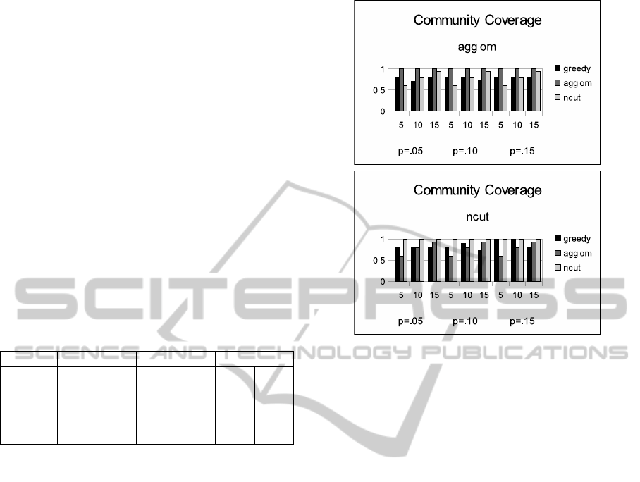
4.4 Community Coverage
The results for the experiments on the community
coverage are presented in Figures 3 to 6. Figure 3
shows the results for the football set. The results are
separated into two charts, the top shows the results for
communities formed by the agglom algorithm and the
bottom one shows the results for ncut.
The charts show the percentage of the communi-
ties that are covered by the activated nodes after the
diffusion process. The bars are grouped first by the
p values of .05, .10 and .15. Within these groups
there is a set of bars for communities of 5, 10 and
Figure 3: Community coverage for football data set.
15. The three bars in each group represent the three
algorithms, greedy, agglom and ncut.
For example, looking at the first set of bars (for
p = .05 and communities=5), greedy covered about
80% of the communities, agglom covered 100% and
ncut covered about 75%. Note that for the agglom
groups, the agglom algorithm always has 100% cov-
erage and for the ncut communities, ncut always has
100% coverage. This is by design, since the algo-
rithms select a node from every community. However,
one of the algorithms (say agglom) may not (and of-
ten does not) do as well covering the communities of
the other community-finding algorithm.
The results in the other figures are organized in the
same way as Figure 3, with Figure 4 for the jazz set,
Figure 5 for the webkb set and Figure 6 for the cora
set.
In analyzing the community coverage results, as
already stated, the algorithm used to find the commu-
nities will always cover 100% of the communities but
what we are interested in is how well the greedy algo-
rithm and the other community-based approach do in
covering them.
In Figure 3, the top chart shows mixed results
where in most cases both greedy and ncut cover be-
tween 60% and 90%. In slightly more than half of the
experiments ncut does better than greedy. In the bot-
tom chart the algorithms do about the same at cover-
ing the ncut groups with agglom doing better in some
cases and greedy doing better in some.
The coverage for the jazz set in Figure 4 has a dif-
DiscoveringInfluentialNodesinSocialNetworksthroughCommunityFinding
409
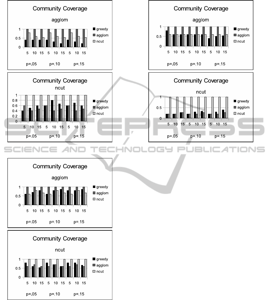
Figure 4: Community coverage for jazz data set.
Figure 5: Community coverage for webkb data set.
ferent look from the football set. In general the al-
gorithms are not as good at covering communities in
the jazz set. In the top chart, the ncut algorithm is
much better at covering the agglom communities than
greedy. However, in the bottom chart the agglom al-
gorithm does worse than greedy at covering the ncut
communities.
Figure 5 appears to reflect the observations made
Figure 6: Community coverage for cora data set.
for the previous two figures. Figure 6 however, ap-
pears to deviate from the other charts. The coverage
of greedy and the other method are about 50% for the
top chart and much below 50% for the bottom.
With all four sets, there is no clear winner between
using greedy and the other method; in trying to cover
unknown communities, there does not seem to be a
advantage to using a community-based method over
a general influence maximization algorithm. The two
algorithms, agglom and ncut find drastically different
types of communities. So it appears that in trying to
cover communities of an unknown type, there may
not be an advantage to using an arbitrary community
finding algorithm.
However, clearly, if one feels as though the un-
derlying community structure of a data set is modeled
after a particular community finding algorithm, then
using that algorithm in a community based approach
to finding influential nodes will almost certainly max-
imize the community coverage.
4.5 Speed Comparisons
Finding communities is a very different task from
finding influential nodes and the algorithms compared
here have very different approaches to the task at
hand. Thus the discussion of complexity in Section
3 was unfortunately unable to give a clear compari-
son of the different methods.
The running time of the experiments performed in
this section were recorded and summarized in Table 3.
WEBIST2013-9thInternationalConferenceonWebInformationSystemsandTechnologies
410

Table 3: Recap of average speedup of agglom and ncut over
greedy.
nodes agglom ncut
football 115 876 876
jazz 198 1908 1882
webkb 877 14 6512
cora 2708 1 27541
The numbers in the table represent the speed up over
the greedy algorithm using the formula speedup =
t
g
t
a
for agglom and speedup =
t
g
t
n
where t
g
, t
a
and t
n
are
the runtimes for greedy,agglom and ncut respectively.
Both algorithms show a profound increase in speed
over greedy for small data sets. For ncut, the increase
becomes more pronounced with a higher number of
nodes. The agglom algorithm, however slows down
relative to greedy as the data sets become larger. With
the cora set they are actually about the same speed.
With larger sets, it is assumed that greedy becomes
faster than agglom.
Two things must be noted. First is that agglom
is a rather slow community finding algorithm. We
chose it because it provides pure ego-centric com-
munities as a contrast to ncut’s purely disjoint com-
munities. Second, there have been many other com-
munity finding algorithms proposed that have a much
better complexity than ncut or agglom. Again these
were chosen to provide a clear contrast between dif-
ferent types of communities and not for speed but it
should be clear that using a community finding algo-
rithm would almost certainly be faster than using the
greedy approach.
5 CONCLUSIONS
Finding influential nodes is an interesting problem
that can be important to managers in marketing, pol-
itics and other diverse areas. Algorithms have been
proposed that find an initial set of nodes to activate in
order to maximize the number of nodes that will be-
come activated after the initial set of nodes are used
in the diffusion model.
The problem itself has been previously shown to
be NP-hard (Clauset et al., 2006). The approximation
algorithms, while tractable are normally quite slow.
They are designed to simply find an initial node set
to maximize the spread of influence. An interesting
extension to the problem is to not only maximize the
spread of influence but to widen the spread by cover-
ing many different communities within the network.
We propose in this paper to use community find-
ing algorithms to not only find a large number of acti-
vated nodes but also to cover as many of the commu-
nities as possible.
We have shown in the experiments that our ap-
proach is competitive in many data sets, with the re-
sults of the traditional greedy algorithm. While the
greedy approach will almost always perform better
using a community finding approach will often per-
form quite well.
The most interesting finding from this study
though, concerns the problem of maximizing the
community coverage. Many network data sets have
an underlying community structure. However, even
if it is known that there is a community structure, the
structure type can vary from one set to another. With-
out knowing what the community structure of a set is,
using a community finding approach is no better than
a typical greedy algorithm for maximizing the com-
munity coverage. However, if an analyst is knowl-
edgeable about the community structure of a set, they
can use a community finding algorithm appropriate
for that set which should maximize the community
coverage.
REFERENCES
Bharathi, S., Kempe, D., and Salek, M. (2007). Compet-
itive influence maximization in social networks. In
Proceedings of WINE.
Chen, W., Wang, Y., and Yang, S. (2009). Efficient influ-
ence maximization in social networks. In Proceedings
of the 15th ACM SIGKDD international conference on
Knowledge discovery and data mining.
Chen, Y. C., Chang, S. H., Chou, C. L., Peng, W. C., and
Lee, S. Y. (2012). Exploring community structures for
influence maximization in social networks. In Pro-
ceedings of SNA-KDD.
Clauset, A., Moore, C., and J.Newman, M. E. (2006). Struc-
tural inference of hierarchies in networks. In Proceed-
ings of the 23rd International Conference on Machine
Learning (ICML), Workshop on Social Network Anal-
ysis.
Domingos, P. and Richardson, M. (2001). Mining the net-
work value of customers. In Proceedings of the Seveth
ACM SIGKDD International Conference on Knowl-
edge Discovery and Data Mining, pages 57–66.
Goldenberg, J., Libai, B., and Muller, E. (2001). Using
complex systems analysis to advance marketing the-
ory development: Modeling heterogeneity effects on
new product growth through stochastic cellular au-
tomata. Academy of Marketing, 01.
Granovetter, M. (1978). Threshold models of collective be-
havior. The American Journal of Sociology, 83.
Jain, A. and Dubes, R. (1988). Algorithms for clustering
data. Prentice-Hall, Inc.
Kempe, D., Kleinberg, J., and Tardos, E. (2003). Maximiz-
ing the spread of influence through a social network.
DiscoveringInfluentialNodesinSocialNetworksthroughCommunityFinding
411

In Proceedings of the Ninth ACM SIGKDD Interna-
tional Conference on Knowledge Discovery and Data
Mining, pages 137–146.
linqs. Statistical relational learning group.
http://www.cs.umd.edu/linqs/.
Narayanam, R. and Narahari, Y. (2011). A shapley value-
based approach to discover influential nodes in social
networks. Automation Science and Engineering, IEEE
Transactions on, 8(1):130 –147.
Newman, M. and Girvan, M. (2004). Finding and evalu-
ating community structure in networks. Physical Re-
view E, 69.
Pearson, M., Steglich, C., and Snijders, T. (2006). Ho-
mophily and assimilation among sport-active adoles-
cent substance users. Connections, 27:47–63.
Porter, M., Onnela, J., and Mucha, P. (2009). Communities
in networks. Notices of the American Mathematical
Society, 56.
Shi, J. and Malik, J. (2000). Normalized cuts and image
segmentation. IEEE Transactions On Pattern Analysis
And Machine Intelligence, 22(8).
Tang, L., Wang, X., Liu, H., and Wang, L. (2010). A multi-
resolution approach to learning with overlapping com-
munities. In KDD Workshop on Social Media Analyt-
ics.
Wang, Y., Cong, G., Song, G., and Xie, K. (2010).
Community-based greedy algorithm for mining top-k
influential nodes in mobile social networks. In Pro-
ceedings of SIGKDD.
WEBIST2013-9thInternationalConferenceonWebInformationSystemsandTechnologies
412
