Power-saving Design in Server Farms for Multi-tier Applications under

Response Time Constraint

Shengquan Wang

, Waqaas Munawar

, Xue Liu

and Jian-Jia Chen

Department of Computer and Information Science, Univ. of Michigan-Dearborn, Dearborn, U.S.A.

Department of Informatics, Karlsruhe Institute of Technology, Karlsruhe, Germany

School of Computer Science, McGill University, Montreal, Canada

Keywords:

Power Saving, Server Farm, Multi-tier, Response Time, Service Level Agreement (SLA), M/G/1/PS, Mean

Value Analysis (MVA).

Abstract:

Server farms suffer from an increasing power consumption nowadays. Power saving has become a prominent

design issue in server farms. This paper presents a power-saving design in server farms under the constraint

of the response time. In particular, we target on multi-tier applications, which are very typical on the web in

modern days. We propose an efﬁcient power-saving design strategy, called

PowerTier

. This strategy exploits

two major techniques by using Dynamic Power management (DPM) to activate/deactivate servers and using

Dynamic Voltage Scaling (DVS) to adjust the processor speed for each activated server. In addition,

PowerTier

considers two different application models: the open-queueing model and the closed-queueing model for

session-less and session-based web applications respectively. With

PowerTier

, we are able to choose the

number of activated servers at each tier and the processor speed for each server to minimize the overall power

consumption in server farms while meeting a given mean response time guarantee for multi-tier applications.

Our comprehensive simulation conﬁrms the effectiveness and efﬁciency of

PowerTier

1 INTRODUCTION

Power has become one of the most dominant oper-

ating cost in server systems. By 2011, data centers

in U.S. are expected to consume around 100 billion

kW per year (U.S. Environmental Protection Agency

(EPA), 2007), in which the annual power cost is

around 7.4 billion US$. Moreover, given the large

number of servers in use today, the worldwide ex-

penditure on enterprise power and cooling of these

servers is estimated to be in excess of 30 billion

US$ (Raghavendra et al., 2008). At the same time,

guaranteeing the performance-oriented Service Level

Agreement (SLA) signed with the clients is critical

to clients’ satisfaction for online business. A com-

mon SLA is deﬁned as (the mean value of) the re-

sponse time constraint, and a delayed response to

clients will have negative effects on online business

including client frustrations and revenue loss. In or-

der to meet a satisfying SLA for an increasing service

demand from clients, server farm becomes a common

practice in industry. A server farm could be composed

of a cluster of tens to thousands of servers to provide

large computing capability. However, the power con-

sumption in server farms is tremendous.

Recently, an increasing attention has been paid on

how to reduce the power consumption while main-

taining a given SLA. In (Rusu et al., 2006), a timing-

aware power management scheme was proposed that

combines cluster-wide, server on/off scheme and lo-

cal power management techniques in heterogeneous

clusters. A new threshold-based approach was pre-

sented in (Wang and Lu, 2008) for efﬁcient power

management of heterogeneous soft real-time clus-

ters in making three important design decisions on

ordered server list, server activation thresholds and

workload distribution. In (Guerra et al., 2008),

a queueing theoretical technique was proposed to

balance energy consumption and adequate applica-

tion response times in heterogeneous CPU-intensive

server clusters. In (Bohrer et al., 2002; Sharma et al.,

2003), low-power opportunities for web servers has

been utilized to reduce the energy consumption by

applying Dynamic Voltage Scaling (DVS) with min-

imal impact on the server performance. A queueing

model was used in (Gandhi et al., 2009) to predict

the optimal power allocation in a variety of scenarios

with DVS and Dynamic Power Management (DPM)

137

Wang S., Munawar W., Liu X. and Chen J..

Power-saving Design in Server Farms for Multi-tier Applications under Response Time Constraint.

DOI: 10.5220/0004357201370148

In Proceedings of the 2nd International Conference on Smart Grids and Green IT Systems (SMARTGREENS-2013), pages 137-148

ISBN: 978-989-8565-55-6

 2013 SCITEPRESS (Science and Technology Publications, Lda.)

by activation/deactivation of servers in both closed-

queueing and open-queueing models. In (Wierman

et al., 2009), an optimal speed scaling was proposed

to balance the mean energy consumption and mean

response time under Processor Sharing (PS) schedul-

ing.

All of these work focused on simple single-tier

applications. As we know, modern web applications

are usually using multi-tier architecture (Kamra et al.,

2004; Liu et al., 2006; Liu et al., 2008; Urgaonkar

et al., 2005; Paciﬁci et al., 2005; Diao et al., 2006;

Liu et al., 2005; Wang et al., 2010). Each tier pro-

vides a certain speciﬁc functionality to applications.

A client request will pass through a series of tiers

to attain a complete service. For instance, a typ-

ical e-commerce application consists of three tiers:

web server tier, application server tier, and database

server tier. The multi-tier architecture follows lay-

ered queueing models (Rolia and Sevcik, 1995) and

typically has a cross-tier dependency. The service at a

tier is normally blocked while waiting for the service

from its succeeding tier. Such cross-tier dependency

makes the response time analysis challenging in com-

parison with the single-tier architecture. In (Liu et al.,

2005), an analytical model was proposed for 3-tiered

web service architecture. The concurrency limit was

addressed in (Urgaonkar et al., 2005) for multi-tier

applications. In (Paciﬁci et al., 2005), an architecture

and underlying model of a performance management

system was presented for multi-tier web applications

on server clusters. In (Diao et al., 2006), a hybrid per-

formance model for differentiated services was pre-

sented for multi-tier applications with cross-tier inter-

action. Among these work, only in (Diao et al., 2006)

the cross-tier dependencywas considered, and the rest

applied a tandem-queue-likestructure and ignored the

cross-tier dependency. In (Wang et al., 2010), an over-

simpliﬁed M/M/1 model is used to perform the queue-

ing analysis in multi-tier architecture.

In this paper, we aim to conduct a comprehen-

sive study on power saving in server farms for multi-

tier applications requiring that a given SLA should

be met. We adopt two techniques as used in server

farms for power-aware design: the DVS technique

with variable speeds and the DPM technique with ac-

tivation/deactivation of servers. There are two spe-

ciﬁc questions that we need to address in the system

design in order to achieve this goal: (i) How many

servers should be activated at each tier? (ii) What is

the best processor speed (corresponding to the volt-

age/frequency to be used) for each server? For a

single-tier architecture with homogeneous servers, it

is shown in (Gandhi et al., 2009) that the optimal

strategy is to set all servers with the same speed for

all activated servers. However, this does not hold in

the multi-tier architecture due to the cross-tier depen-

dency. We present an efﬁcient power-saving design

strategy called

PowerTier

and study how to choose

the number of activated servers at each tier and the

processor speed for each server to minimize the over-

all power consumption in server farms while meeting

a given mean response time guarantee for multi-tier

applications. We consider both open-queueing and

closed-queueing models for applications.

The rest of this paper is organized as follows: Sec-

tion 2 shows the system model. Section 3 presents a

detailed power consumption and response time anal-

ysis, which is the basis for our power-saving design.

Our power-saving design scheme

PowerTier

is de-

scribed in Section 4. Section 5 presents detailed per-

formance evaluation of

PowerTier

over a various of

platforms. We conclude the paper in Section 6.

2 SYSTEM MODEL

In this section, we deﬁne the system model, including

the power consumption model for servers, the multi-

tier architecture, and the client application model.

2.1 Power Consumption Model

We assume that all servers are equipped with the

DVS and DPM techniques for the power manage-

ment. When the server is deactivated by the DPM

technique, its power consumption is negligible. So,

here we focus on the power consumption when the

server is activated.

With the DVS technique, we can choose a proces-

sor speed for a server (with a corresponding choice of

the supply voltage). We deﬁne r as the ratio of the

processor speed of the server to its maximum speed.

The speed ratio r is normally bounded by a lower

bound r

. Then we haver

≤ r ≤ 1. When the server is

activated, either it is (i) in the idle mode at the lowest

speed ratio r

without executing any job; or (ii) in the

running mode executing jobs with a processor speed

ratio r. The power consumption in our study is the

system-level power, including the power consumed

by the processor and all other components within the

server such as memory and I/O devices. The power

consumption depends on the mode that the server is

in (idle or running) and the processor speed in use as

well. In this paper, we adopt the power consumption

model in (Gandhi et al., 2009). A server has the fol-

lowing power modes:

• Idle Power Mode. In the idle mode, the server

consumes the static power P

;

SMARTGREENS2013-2ndInternationalConferenceonSmartGridsandGreenITSystems

138

• Running Power Mode. In the running mode, the

power consumption P

(r) by the server at a speed

ratio r is

(r) = α[r− r

]

+ P

, (1)

where γ ≥ 1. The cubic rule is widely suggested

in the literature for the processor power-to-speed

relationship in the running mode, i.e., γ = 3. How-

ever, in server farms with DVS or for some appli-

cations, the linear rule could be applied (Gandhi

et al., 2009).

The different power modes provide the space for

system designers to design efﬁcient power-saving

strategies.

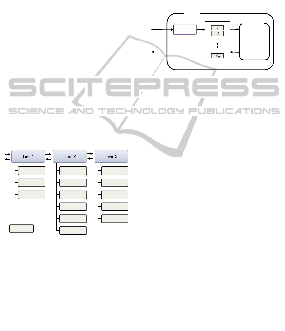
2.2 Multi-tier Architecture

We consider a system with M tiers, each of which

consists of a server farm. We assume that all tiers

run on homogeneous servers. Tier m has v

activated

servers and each runs at a speed ratio r

. The homo-

geneous sever assumption was used in previous simi-

lar studies (Gandhi et al., 2009).

We assume a pro-

cessor sharing (PS) scheduling at each server, since it

approximates well the scheduling algorithms used by

most commodity operating systems such as Linux.

Tier 1 Tier 2! Tier 3!

server

Figure 1: A three-tier architecture with 3 servers at Tiers 1,

7 servers at Tier 2, and 6 servers at Tier 3.

Figure 1 illustrates a three-tier architecture. A

client starts a request at the outer tier, denoted as Tier

1, and then goes to an inner Tier m (m≥ 2) one by one

if necessary. When a request arrives at Tier m, it trig-

gers one or more requests at its succeeding Tier m+1.

After some processing at Tier m, it either returns to

Tier m− 1 or proceeds to Tier m+ 1. The exceptions

are the last Tier M, where all requests return to the

Tier M − 1, and the ﬁrst Tier 1, where returning to

the preceding queue means request completion. This

We can extend it to the heterogeneous case by taking

into consideration the different characteristics of servers.

model can handle multiple visits to a tier including se-

quential and parallel accesses (Diao et al., 2006). We

denote κ

m+1

as the average request visit ratio at Tier

m+ 1 by a request at Tier m. If we deﬁne λ

as the

request arrival rate at Tier m

, then we have

m+1

. (2)

Tier m

Tier m+1



Server farm

1

2

dispatcher

Figure 2: Cross-tier dependency.

The system supports many clients. At each tier, a

dispatcher (or load balancer) as shown in Figure 2 will

distribute all incoming requests from clients to one of

the servers in the server farm of this tier. We assume

that they are evenly distributed to the servers at each

tier. The multi-tier architecture shows a cross-tier de-

pendency (Diao et al., 2006; Rolia and Sevcik, 1995).

It could be illustrated with a nested structure in Fig-

ure 2, where Tier m includes the succeeding Tierm+1

for m < M. A request can only be completed at each

tier after it has received service from the succeeding

tier (if it needs service from the succeeding tier). We

assume that the waiting for the outcome from the suc-

ceeding tier is non-blocking, i.e., the waiting process

will not block other processes in the same server from

using the resources such as CPU during its waiting.

2.3 Client Application Model

Applications for clients could be session-less or

session-based. Each session-less application issues

one request during its life while a session-based ap-

plication usually issues more requests during its life-

time with think times in between and normally lasts

for a while. The former can be modeled as an open-

queueing system and the latter as a closed-queuing

system (Jain, 1991). In an open-queueing system, ap-

plications start and end even though we could assume

a ﬁxed average arrival rate, but in a closed-queueing

system, applications stay and the number of the ses-

sions remains the same. Figure 3 shows open/closed-

queueing models at Tier 1. For the closed-queueing

model, we deﬁne N

delay servers, each of which cor-

responds to the think time for each session at Tier 1

In the closed-queueing model introduced later, λ

is de-

ﬁned as throughput since the number of sessions is ﬁxed.

Power-savingDesigninServerFarmsforMulti-tierApplicationsunderResponseTimeConstraint

139

Tier 1



!"#$%&'()%)%*+,-

./%+'()%)%*+,-

Figure 3: Open-queueing and closed-queueing models at

Tier 1.

(Liu et al., 2005).

In the multi-tier architecture, the system could

be decoupled into subsystems by tiers. In either

open-queueing or closed-queueing model, at Tier m

(m ≥ 2), none, one, or more requests could be gen-

erated with ratio κ

after the proceeding tier. In the

study of server performance, M/G/1/PS server model

has been shown by different research studies that can

model the open-queueing servers well (Kamra et al.,

2004; Wang and Lu, 2008; Gandhi et al., 2009; Wier-

man et al., 2009; Liu et al., 2008; Liu et al., 2006;

Heo et al., 2007). Mean Value Analysis (MVA) is

widely used in closed-queueing servers (Lazowska

et al., 1984; Jain, 1991; Reiser and Lavenberg, 1980)

for response time analysis.

3 POWER CONSUMPTION AND

RESPONSE TIME ANALYSIS

Recall that our objective is to minimize the power

consumption under the mean response time con-

straint. First we need to conduct the power consump-

tion and response time analysis. We start it with single

server, then we extend it to server farm in a multi-tier

architecture.

3.1 Single Server

Power Consumption. We consider a server that

will switch in two power modes alternatively: running

and idle. We deﬁne π

and π

as the probabilities that

the server is in running and idle mode respectively,

where π

+ π

= 1, then the mean power consump-

tion can be written as:

E[P] = P

(r)π

+ P

= α[r− r

]

+ P

, (3)

where P

(r) is deﬁned in (1). According to (3), in

order to calculate the mean power, we need to obtain

the value of π

• For an open-queueing M/G/1/PS server, if re-

quests are with an arrival rate λ, and a general-

ized service time distribution with a given mean

value E[S], then by the traditional queueing the-

ory (Kleinrock, 1976) we have

= λE[S]. (4)

• For a closed-queueing server, we could use the

same formula in (4) to calculate π

. However λ

in (4) should be throughput instead

. Assume

that there are N ﬁxed number of sessions, jobs are

with a mean response time E[R], and a mean think

time E[Z] in between, then by (Jain, 1991), the

throughput λ can be obtained as

λ =

E[R] + E[Z]

, (5)

where E[R] is to be determined.

Response Time Analysis. The response time is de-

ﬁned as the time spent by a job in waiting in the queue

and executing on the processor.

• For an open-queueing M/G/1/PS server, by the

traditional queueing theory (Kleinrock, 1976), the

mean response time is

E[R] =

E[S]

1− λE[S]

. (6)

• For a closed-queueing server, we use MVA to ob-

tain the mean response time (Jain, 1991). We de-

ﬁne D(N) as the mean delay for N sessions. D

can be calculated recursively in terms of N. If we

denote Q(N) as the mean queue length with N ses-

sions, then with MVA we have

D(N) = [Q(N − 1) + 1]E[S], (7)

Q(N) =

E[R] + E[Z]

D(N), (8)

where Q(0) = 0. To reduce the computa-

tion complexity, we could use the well-accepted

Schweitzer’s approximation (Jain, 1991) by ap-

proximating Q(N − 1) ≈

N−1

Q(N) to avoid the

recursive computation. Then D(N) will be the

positive solution to the following equation:

D(N) =



[N − 1]D(N)

E[R] + E[Z]

+ 1



E[S], (9)

where the response time E[R] = D(N) for single

tier.

The analysis in single server regarding power con-

sumption and response time will be the basis for

server farms in a multi-tier architecture.

The throughput is equivalent to the arrival rate in open-

queueing model and so we use the same notation λ.

SMARTGREENS2013-2ndInternationalConferenceonSmartGridsandGreenITSystems

140

3.2 Server Farm in Multi-tier

Architecture

In the following, we consider the multi-tier architec-

ture with each tier having multiple servers. We add

a subscript m into the terms introduced above for any

server at Tier m.

We assume that the average service demand is

ﬁxed in the system, which is the arrival rate λ

and

the number of sessions N

at Tier 1 for open/closed-

queueing models respectively. By (5), the throughput

at Tier 1 in closed-queueing model can be written as

E[R

] + E[Z]

, (10)

where E[R

] is to be determined.

At Tier m (m = 1, 2, . . . , M), given the visit ratio

and the number v

of the servers, the request ar-

rival rate can be obtained as

= λ

[

∏

i=1

]. (11)

Recall that Tier m has v

homogeneous servers. Since

the arrival is evenly distributed to each server at each

tier, the arrival rate at any server at Tier m is

Power Consumption. In order to calculate the

mean power for servers at each tier, we need to ﬁnd

R,m

, i.e., the probability that a server at Tier m is in

the running mode. We assume that the server is in the

idle power mode when it is waiting for the outcome

from the succeeding tier. For either an open-queueing

or closed-queueing server at Tier m, we have

R,m

E[S

], (12)

where λ

is deﬁned in (11). The value of λ

in (11)

is given for an open-queueing server and deﬁned by

(10) for a closed-queueing server respectively. Then

applying (12) into (3), we can obtain the mean power

consumption.

Response Time Analysis. In multi-tier architec-

ture, the response time analysis is more complex due

to the cross-tier dependency. The response time at

each tier also includes the waiting time for the out-

come from the succeeding tier, which is κ

m+1

E[R

m+1

]

at Tier m (Diao et al., 2006). Recall that the wait-

ing for the outcome from the succeeding tier is non-

blocking. Then applying this observation into (6) and

(7), we have the following results:

• For an open-queueing M/G/1/PS server at Tier m,

the response time is

E[R

] =

E[S

]

1−

E[S

]

+ κ

m+1

E[R

m+1

], (13)

where λ

is deﬁned in (11).

• For a closed-queueing server at Tier m, we denote

as the mean delay experienced by any server at

Tier m. The hit ratio for any session at any server

at Tier m is [

∏

j=1

]

(Urgaonkar et al., 2005).

Then with the approximated MVA in (9), the re-

sponse time for any request at Tier m is

E[R

] = D

+ κ

m+1

E[R

m+1

], (14)

which satisﬁes

− 1][

∏

j=1

]

E[R

] + E[Z]

+ 1

E[S

(15)

We assume the mean service time for a server at

Tier m is E[S

] =

under the maximum speed. If

the server runs at a speed ratio r

in the running mode,

we have E[S

] =

. Applying this into the above

results, we have the complete analysis of power con-

sumption and response time for server farms in multi-

tier architecture. It is summarized in the following

theorem:

Theorem 1. We consider both open/closed-queueing

models for server farms in multi-tier architecture. For

either an open-queueing or closed-queueing server at

Tier m, the mean power consumption is

E[P

] =

α[r

− r

]

+ P

, (16)

where λ

is deﬁned in (11). The mean response time

of a job can be obtained as follows:

• For an open-queueing M/G/1/PS server at Tier m,

the mean response time of a job is

E[R

] =

−

+ κ

m+1

E[R

m+1

], (17)

for m = 1, 2, . . . , M with R

M+1

= 0.

• For a closed-queueing server at Tier m, the mean

response time of a job is

E[R

] = D

+ κ

m+1

E[R

m+1

], (18)

which satisﬁes

− 1][

∏

j=1

]

E[R

] + E[Z]

+ 1

(19)

In the above formulas, λ

and N

are given for

open/closed-queueing server respectively.

We notice that in closed-queueing model, D

’s

depends on each other by (18) and (19). Such

inter-dependency among D

’s generates an implicit

formula for the response time analysis in closed-

queueing model. In such case, we could use the clas-

sical ﬁxed point theorem to solve it.

Power-savingDesigninServerFarmsforMulti-tierApplicationsunderResponseTimeConstraint

141

PowerTier

: AN EFFICIENT

POWER-SAVING DESIGN

In this section, we will study our power-saving design

strategy

PowerTier

for server farms in multi-tier ar-

chitecture. The power-saving design could be divided

into two phases:

• Planning or upgrading: In this phase, we could

determine the number of servers (denoted as ˆv

)

needed for the peak service demand which is

deﬁned as the maximum arrival rate and the

maximum number of sessions at Tier 1 for

open/closed-queueing models respectively (de-

noted as

and

respectively).

• Runtime: In this phase, the number of the avail-

able servers are ﬁxed, which were obtained in the

planning or upgrading phase. For any level of ser-

vice demand, we will decide how many servers

should be activated/deactivated and the processor

speed for each server.

In each phase, we assume that the visit ratio κ

’s

and the service rate µ

’s were learned through the

monitored history, and so they are known in the de-

sign. The major difference between these two phases

is that we can switch servers among different tiers in

the planning or upgrading phase, but not practically

in the runtime phase.

In our design, we aim to minimize the mean power

consumption under a given mean response time con-

straint, where we choose a mean responsetime thresh-

old

R. For given service demand λ

and N

(in

open/closed-queueing model respectively), we need

to determine the number of the activated servers at

each tier and the processor speed of each activated

server, i.e., the value of v

and r

for m = 1, 2, . . . , M.

The optimization problem can be formulated as fol-

lows:

min

:m=1,2,...,M}

E[P] =

∑

m=1

E[P

] (20a)

subject to E[R] = E[R

] ≤

R, (20b)

max{r

} ≤ r

≤ 1, (20c)

1 ≤ v

≤ ˆv

. (20d)

Inequality (20c) is based on the bound of r

≤

≤ 1) and the stability condition of a server (r

). Inequality (20c) is the server availability con-

straint. Notice that we will only have the lower bound

in the planning or upgrading phase.

In the planning or upgrading phase, if the number of

the overall available servers are limited due to budget, we

need to add this additional constraint too.

In order to solve the above optimization with non-

linear constraints, we ﬁrst treat v

as continuous val-

ues to deal with the integer programming. Since all

E[P

] and E[R

] are convex functions in terms of

and v

, the optimization problem can be solved

with the Lagrangian method. We deﬁne the Lagrange

equation L with the Lagrange multipliers φ and χ

k,m

(k = 1, 2, 3 and m = 0, 1, . . . , M) as

L =

∑

m=1

E[P

] + φE[R

] +

∑

m=1

[χ

1,m

− r

][r

− 1]

− χ

2,m

− 1][v

− ˆv

] − χ

3,m

], (21)

where all multipliers are non-negative.

We set

∂L

∂r

= 0 and

∂L

∂v

= 0 for m = 1, 2, . . . ,M.

Together with equalities in (13) and the following

equalities

φ[E[R

] −

R] = 0, (22)

1,m

− r

][r

− 1] = 0, (23)

2,m

− 1][v

− ˆv

] = 0, (24)

3,m

[λ

− r

] = 0, (25)

we can solve the values of the variables.

The key in the above equations is to solve

∂L

∂r

= 0

and

∂L

∂v

= 0 for m= 1, 2, . . ., M. Given the power con-

sumption and response time analysis summarized in

previous section for both open/closed-queueing mod-

els, we can obtain the formula.

We denote r

∗

and v

∗

as the obtained optimal r

and v

respectively. Since v

∗

’s are integer values, we

could choose their rounded-up values as the ﬁnal out-

put. Then apply the rounded-up v

∗

into the above op-

timal approach with ﬁxed server allocation and obtain

the ﬁnal solution.

We summarize the main result in the following

theorem:

Theorem 2. Given κ

’s, µ

’s, λ

(in the open-

queueing model) and N

(in the closed-queueing

model), with the

PowerTier

design we could ﬁnd

the (heuristically) optimal values r

∗

and v

∗

(m =

1, 2, . . ., M) such that the power consumption can be

minimized as E[P

∗

] while the mean response time

E[R

] is below the mean response time threshold

With the

PowerTier

design, we determine server

allocation at each tier for the planning or upgrading

phase for the peak service demand. Also, for the

running phase, for different service demands and the

visit ratios, we also determine the number of acti-

vated/deactivated servers at each tier and the proces-

sor speed for each activated server. With the

Pow-

erTier

design, we are able to minimize the mean

power consumption under the given mean response

time constraint.

SMARTGREENS2013-2ndInternationalConferenceonSmartGridsandGreenITSystems

142

5 PERFORMANCE EVALUATION

In this section, we ﬁrst verify the queueing analysis in

multi-tier architecture in both open/closed-queueing

model as shown in Section 3. Then we present perfor-

mance evaluation of our proposed

PowerTier

design.

5.1 Verifying Queueing Analysis in

Multi-tier Architecture

We employed the RUBiS (Cecchet et al., 2002) sys-

tem to generate and analyze the trafﬁc for measur-

ing the timing parameters. The RUBiS system offers

an eBay like web service with an associated client

to generate the test trafﬁc. It is a three-tier hierar-

chical system with a possibility of having more than

one server per tier. First tier consists of Apache

load balancer, the second includes the JBoss applica-

tion server and the third consists of MySQL database

server. We allocated one physical machine per tier.

For the purpose of evaluation, we modiﬁed two as-

pects of RUBiS’ test trafﬁc generator: (i) it was al-

tered to record a complete trace of the requests and

wrote an additional tool to replay the saved trace. This

helps negate the effects of any probabilistic ﬂuctua-

tions arising from differences in the traces. (ii) Sec-

ondly, we instrumented the RUBiS server side code

to measure the inter tier request ratios and per tier re-

sponse times. Overall, this architecture to measure

the empirical results, insured accurate emulation of

an actual typical multi-tier web service.

We obtained the mean service time at the

maximum speed at each tier as (

) =

(1.2, 6.86, 5.43) ms, and the visit ratio as

(κ

, κ

) = (1, 1, 1.24074), and adopted the think

time 0.035 sec in the closed-queueing model, which

is used in (Liu et al., 2005). The available frequencies

for each server are: the Apache server – 3.0GHz

and 2.8GHz; the JBoss server – 3.1, 3.0, . . . , 1.6GHz;

the MySQL server – 2.13GHz, 1.87GHz, and

1.60GHz. We consider two kinds of conﬁgurations

of frequencies at tiers: (3.0, 3.1, 2.13)GHz and

(2.8, 2.5, 1.6)GHz.

We have run over 5, 000 requests and ﬁxed the ar-

rival rate λ

= 8.862, 17.723 per second for the open-

queueing model. We measure the mean response time

for each request at each tier and compare it with the

modeled one. The results are shown in Table 1. In all

cases, the maximum error of measured response time

compared with the modeled one is 4% and most of

them are pretty small. It shows that the modeling is

pretty accurate.

Table 1: Comparison of Measured/Modeled Response Time

in Open-Queueing Model.

(a) λ

= 8.862 and (r

, r

) = (1, 1,1)

E[R

] E[R

]

Measured 16.50 ms 14.72 ms 5.83 ms

Modeled 15.93 ms 14.55 ms 5.83 ms

Error 3.6% 1.2% 0.0%

(b) λ

= 17.723 and (r

, r

) = (1, 1,1)

E[R

] E[R

]

Measured 18.27 ms 16.49 ms 6.71 ms

Modeled 17.72 ms 16.14 ms 6.71 ms

Error 3.1% 2.2% 0.0%

= 8.862 and (r

, r

) = (0.90, 0.81, 0.75)

E[R

] E[R

]

Measured 18.27 ms 16.49 ms 6.71 ms

Modeled 17.71 ms 16.37 ms 6.71 ms

Error 3.2% 0.8% 0.0%

(d) λ

= 17.723 and (r

, r

) = (0.90, 0.81,0.75)

E[R

] E[R

]

Measured 21.38 ms 19.63 ms 8.24 ms

Modeled 20.86 ms 18.89 ms 8.24 ms

Error 2.5% 4.0% 0.0%

5.2 Evaluating

PowerTier

Servers. We use three types of servers to evalu-

ate the performance of

PowerTier

: the one as a JBoss

server in the previous experiment, and the other two

from (Gandhi et al., 2009). The one in the previous

experiment is an Intel i3 dual core processor based

server with 6GB of RAM. The server is equipped

with DVFS capability with option to switch between

16 frequencies between 1.6GHz and 3.1GHz. We

enable one core of each server. We measure the

power consumption for the one in the previous ex-

periment. Based on the measured power, we use

Least Squares Fitting to obtain the modeled power

as shown in Figure 4. The power proﬁles of all

three types of servers in Table 2, where Type-B is

the one in the previous experiment. We consider

the same three-tier architecture used in the previous

experiment. We adopt from (Liu et al., 2005) the

mean service time at the maximum speed at each tier

with (

) = (1.2, 15.1, 36.7) ms, the visit ra-

tio (κ

, κ

) = (1, 0.998, 1.603), and the think time

with 0.035 sec in the closed-queueing model.

We scale the job service time for all three type

servers so that the mean service time at the maximum

speed at each tier follows the above speciﬁcation.

Baseline Design Strategies. We consider two base-

line design strategies: (i)

EvenDist

: All servers are

Power-savingDesigninServerFarmsforMulti-tierApplicationsunderResponseTimeConstraint

143

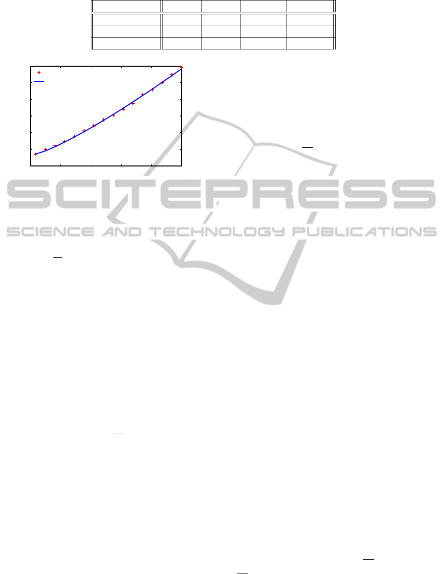
Table 2: Server proﬁles.

γ r

α (Watt) P

(Watt)

Type-A server 1 0.4 100 180

Type-B server 1.2137 0.5161 12.3977 36.7040

Type-C server 3 0.4 455 150

0.5 0.6 0.7 0.8 0.9 1

speed ratio r

Power consumption (Watt)

Measured power

Modeled power

Figure 4: Measured and modeled power.

evenly assigned to 3 tiers. All tiers will almost have

the same number of servers with at most 1-server dif-

ference. (ii)

PropDist

: All servers are proportionally

assigned to 3 tiers according to the absolute utilization

of the tier, i.e.,

. In each baseline, all servers are al-

ways activated with the maximum processor speed,

i.e., r

= 1. An optimization approach similar to pre-

vious section to ﬁnd the minimum required servers

for each baseline. For

PowerTier

, we use the result in

Section 4 to determine the v

∗

at each tier and r

∗

for

each server.

Evaluation in the Planning or Upgrading Phase.

First we determine the optimal number of servers al-

located to each tier for the peak service demand in

the planning or upgrading phase. We consider the fol-

lowing peak service demand: in the open-queueing

model, the maximum arrival

at Tier 1 is 800 per

second; in the closed-queueing model, the maximum

number of sessions

at Tier 1 is 200. The response

time constraint is ﬁxed as

R =

200

= 0.24 sec. Table 3

shows the resulting server allocation and the corre-

sponding speed assignment for each design strategy.

We observe that

EvenDist

needs signiﬁcantly

more processors than the others in all cases. The

server assignment at each tier for

PowerTier

and

PropDist

are pretty similar in all cases. In other

words, the optimal design under peak demand may

adopt proportional server allocation at tiers.

Pow-

erTier

might need extra more servers than

PropDist

(as shown in Type-C Server) since the enable DVFS

PowerTier

could use more servers with lower speed

to reduce power consumption while

PropDist

always

uses the highest speed.

Evaluation in the Running Phase. Second we

compare the performance of

PowerTier

with the base-

line design strategies for the running phase in the fol-

lowing two scenarios:

5.2.1 Fixed Mean Response Time Constraint

In this experiment, we ﬁx the mean response time

constraint as

R =

200

= 0.24 second. We conduct

evaluation in both open/closed-queueing models.

In the open-queueing model, we vary λ

from 0 to

800 per second and choose different types of servers.

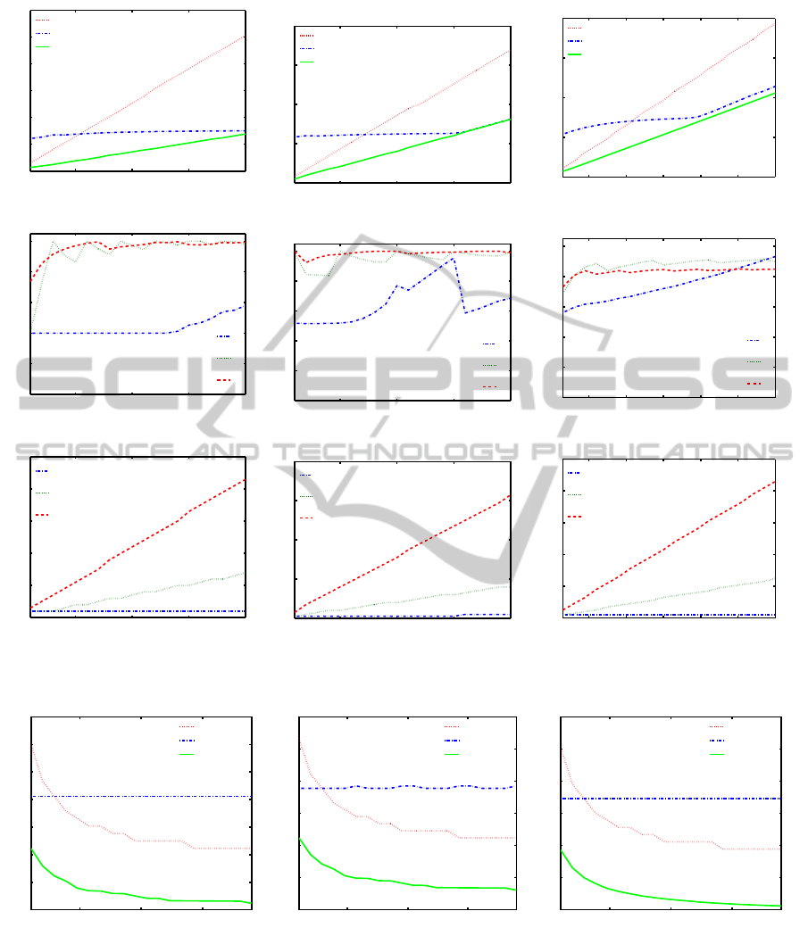
The results are shown in Figure 5. In the closed-

queueing model, we vary N

from 0 to 200 and choose

different types of servers. Similarly, we obtain the re-

sults as shown in Figure 6.

The subﬁgures in the ﬁrst, second, and third rows

are the optimal power consumption for all design

strategies, and the corresponding optimal r

∗

and v

∗

for

PowerTier

respectively. The different columns

are the cases for all three type servers. All the

sawtooth-shaped processor curves are due to the re-

optimization with the consideration of the integer

value of v

∗

PowerTier

Both open/closed-queueing models reveal the

similar phenomenon. In all the cases

PowerTier

out-

performs the others. Both the power consumption

under

PowerTier

and

EvenDist

seem linearly pro-

portionally to the trafﬁc arrival rate (in the open-

queueing model) or the number of sessions (in the

closed-queueing model). But the increasing slope for

EvenDist

is larger. For

PropDist

, when the trafﬁc is

not heavy, it consumes signiﬁcant amount of power

due to the constraint of the proportional distribution

with at least one server at each tier. When the trafﬁc

is heavy,

PropDist

approaches to the optimal design

PowerTier

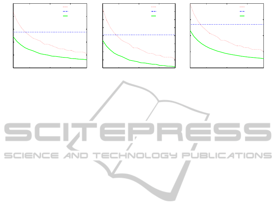
5.2.2 Fixed Service Demand

In this experiment, we ﬁx the service demand and

vary the response time constraint. We also conduct

evaluation in both open/closed-queueing models. We

ﬁx the service demand intensity as 25% with respect

to the peak one, and vary

R from

100

= 0.12 second

400

= 0.48 second.

In the open-queueing model, we choose the re-

quest arrival rate as λ

= 200 per second. Figure 7

SMARTGREENS2013-2ndInternationalConferenceonSmartGridsandGreenITSystems

144

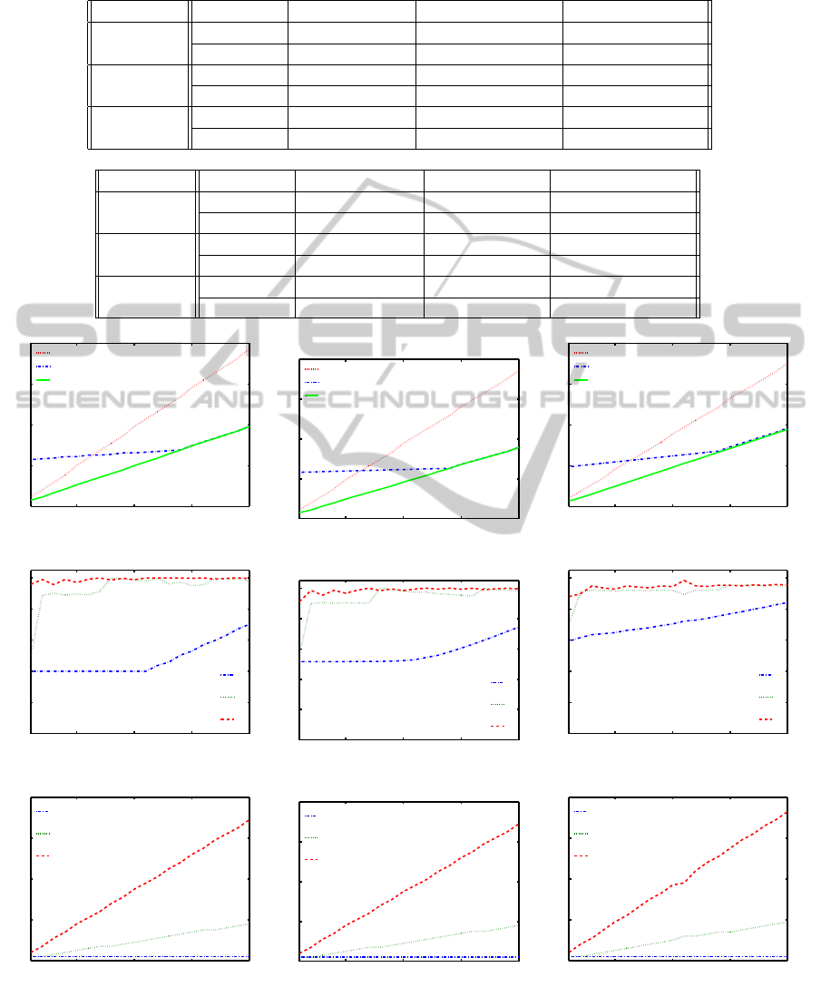
Table 3: Server allocation and processor speed assignment in the planning or upgrading phase.

(a) Open-Queueing Model

Strategies Type-A Server Type-B Server Type-C Server

PowerTier

, v

) (2, 18, 69) (2, 18, 69) (2, 19, 73)

, r

) (0.7, 0.98, 1) (0.74, 0.98, 0.99) (0.84, 0.95, 0.95)

EvenDist

, v

) (65, 65, 65) (65, 65, 65) (65, 65, 65)

, r

) (1, 1, 1) (1, 1, 1) (1, 1, 1)

PropDist

, v

) (2, 18, 69) (2, 18, 69) (2, 18, 69)

, r

) (1, 1, 1) (1, 1, 1) (1, 1, 1)

(b) Closed-Queueing Model

Strategies Type-A Server Type-B Server Type-C Server

PowerTier

, v

) (2, 16, 63) (2, 16, 63) (2, 17, 67)

, r

) (0.63, 1, 0.99) (0.69, 1, 0.99) (0.81, 0.95, 0.95)

EvenDist

, v

) (59, 59, 59) (59, 59, 59) (59, 59, 59)

, r

) (1, 1, 1) (1, 1, 1) (1, 1, 1)

PropDist

, v

) (2, 16, 63) (2, 16, 63) (2, 16, 63)

, r

) (1, 1, 1) (1, 1, 1) (1, 1, 1)

200 400 600 800

E [P

∗

] (kW)

EvenDist

PropDist

PowerTier

200 400 600 800

0.2

0.4

0.6

0.8

∗

200 400 600 800

∗

(a) Type-A Servers

200 400 600 800

E [P

∗

] (kW)

EvenDist

PropDist

PowerTier

200 400 600 800

0.2

0.4

0.6

0.8

∗

200 400 600 800

∗

(b) Type-B Servers

200 400 600 800

E [P

∗

] (kW)

EvenDist

PropDist

PowerTier

200 400 600 800

0.2

0.4

0.6

0.8

∗

200 400 600 800

∗

Figure 5: Comparison in the open-queueing model for

R = 0.24 second.

Power-savingDesigninServerFarmsforMulti-tierApplicationsunderResponseTimeConstraint

145

50 100 150 200

E [P

∗

] (kW)

EvenDist

PropDist

PowerTier

50 100 150 200

0.2

0.4

0.6

0.8

∗

50 100 150 200

∗

(a) Type-A Servers

50 100 150 200

E [P

∗

] (kW)

EvenDist

PropDist

PowerTier

50 100 150 200

0.2

0.4

0.6

0.8

∗

50 100 150 200

∗

(b) Type-B Servers

50 100 150 200 250 300

E [P

∗

] (kW)

EvenDist

PropDist

PowerTier

50 100 150 200 250 300

0.2

0.4

0.6

0.8

∗

50 100 150 200 250 300

100

∗

Figure 6: Comparison in the closed-queueing model for

R = 0.24 second.

0.2 0.3 0.4

R (sec)

E [P

∗

] (kW)

EvenDist

PropDist

PowerTier

(a) Type-A Servers

0.2 0.3 0.4

0.5

1.5

2.5

3.5

R (sec)

E [P

∗

] (kW)

EvenDist

PropDist

PowerTier

(b) Type-B Servers

0.2 0.3 0.4

R (sec)

E [P

∗

] (kW)

EvenDist

PropDist

PowerTier

Figure 7: Comparison in the open-queueing model for λ

= 200 per second.

shows the power consumption comparison. In the

closed-queueing model, we choose the number of ses-

sions as N

= 50. Similarly, we obtain the results as

shown in Figure 8.

In all design strategies, as

R increases, the power

consumption reduces. When

R is very small, i.e.,

the timing requirement is more stringent, then more

servers will be activated, which consumes more

power.

PowerTier

alway outperforms the others. For

larger response time threshold

EvenDist

outforms

PropDist

. For smaller response time threshold

PropDist

outforms

EvenDist

SMARTGREENS2013-2ndInternationalConferenceonSmartGridsandGreenITSystems

146

0.2 0.3 0.4

R (sec)

E [P

∗

] (kW)

EvenDist

PropDist

PowerTier

(a) Type-A Servers

0.2 0.3 0.4

0.5

1.5

2.5

3.5

4.5

R (sec)

E [P

∗

] (kW)

EvenDist

PropDist

PowerTier

(b) Type-B Servers

0.2 0.3 0.4

R (sec)

E [P

∗

] (kW)

EvenDist

PropDist

PowerTier

Figure 8: Comparison in the closed-queueing model for N

= 50.

6 CONCLUSIONS AND FUTURE

WORK

In this paper, we have explored power-saving de-

sign on server farms running multi-tier web appli-

cations under a given SLA. We proposed an efﬁ-

cient power-saving design strategy

PowerTier

, which

jointly considers both DVS and DPM power-saving

techniques. Speciﬁcally, we have considered two ap-

plication models: the open-queueing model and the

closed-queueing model for session-less and session-

based web applications respectively. With

PowerTier

we are able to optimally determine the number of

servers needed at each tier for the peak service de-

mand in the planning or upgrading phase. And also

in the running phase, for different service demands

and request visit ratios, we are able to optimally de-

termine the number of activated/deactivated servers at

each tier and the processor speed for each activated

server. The simulation results showed that

PowerTier

is able to efﬁciently save the power consumption of

server farms while meeting the response time con-

straint for multi-tier applications. Our simulation has

also showed that the optimal server allocation under

the open-queueing and closed-queueing models are

quite different due to the different application behav-

iors.

This paper focused on homogeneous servers at

each tier. One of potential future work is to extend the

current work to heterogeneous servers by taking into

consideration the different characteristics of servers in

the power consumption and response analysis. How-

ever, the optimal design is much more complex and

challenging in this case. This paper also targets on the

stable workload. In the future work, we would like to

exploit a control mechanism to activate and deactivate

servers dynamically. The control period is assumed to

be sufﬁciently long to pay off the energy and timing

overhead of the activation and deactivation of servers.

ACKNOWLEDGEMENTS

This work is sponsored in part by NSF CAREER

Grant No. CNS-0746906, Baden Wuerttemberg

MWK Juniorprofessoren-Programms, NSERC Dis-

covery Grant 341823, FQRNT grant 2010-NC-

131844, CFI Leaders Opportunity Fund 23090, and

National Science Foundation Award 1116606 and

1117664.

REFERENCES

Bohrer, P., Elnozahy, E., Keller, T., Kistler, M., Lefurgy, C.,

McDowell, C., and Rajamony, R. (2002). The case

for power management in web servers. Power Aware

Computing, pages 261–289.

Cecchet, E., Marguerite, J., and Zwaenepoel, W. (2002).

Performance and scalability of EJB applications.

ACM Sigplan Notices, 37:246–261.

Diao, Y., Hellerstein, J., Parekh, S., Shaikh, H., Surendra,

M., and Tantawi, A. (2006). Modeling differentiated

services of multi-tier web applications. In IEEE Inter-

national Symposium on Modeling, Analysis, and Sim-

ulation.

Gandhi, A., Harchol-Balter, M., Das, R., and Lefurgy, C.

(2009). Optimal power allocation in server farms. In

ACM SIGMETRICS.

Guerra, R., Leite, J., and Fohler, G. (2008). Attaining

soft real-time constraint and energy-efﬁciency in web

servers. In ACM symposium on Applied computing.

Heo, J., Henriksson, D., Liu, X., and Abdelzaher, T. (2007).

Integrating adaptive components: An emerging chal-

lenge in performance-adaptive systems and a server

farm case-study. In IEEE Real-Time Systems Sympo-

sium.

Jain, R. (1991). The art of computer systems performance

analysis: techniques for experimental design, mea-

surement, simulation, and modeling. John Wiley &

Sons Inc.

Kamra, A., Misra, V., and Nahum, E. (2004). Yaksha: a

self-tuning controller for managing the performance

Power-savingDesigninServerFarmsforMulti-tierApplicationsunderResponseTimeConstraint

147

of 3-tiered web sites. In IEEE International Workshop

on Quality of Service.

Kleinrock, L. (1976). Queueing Systems Volume II: Com-

puter applications. Wiley Interscience.

Lazowska, E., Zahorjan, J., Graham, G., and Sevcik, K.

(1984). Quantitative system performance: com-

puter system analysis using queueing network models.

Prentice-Hall, Inc. Upper Saddle River, NJ, USA.

Liu, X., Heo, J., and Sha, L. (2005). Modeling 3-tiered web

applications. In IEEE International Symposium on

Modeling, Analysis, and Simulation of Computer and

Telecommunication Systems, 2005, pages 307–310.

Liu, X., Heo, J., Sha, L., and Zhu, X. (2006). Adaptive

control of multi-tiered web applications using queue-

ing predictor. In IEEE/IFIP Network Operations and

Management Symposium.

Liu, X., Heo, J., Sha, L., and Zhu, X. (2008). Queueing-

model-based adaptive control of multi-tiered web ap-

plications. IEEE Transactions on Network and Service

Management, 5(3):157–167.

Paciﬁci, G., Segmuller, W., Spreitzer, M., Steinder, M.,

Tantawi, A., and Youssef, A. (2005). Managing the

response time for multi-tiered web applications. Tech-

nical Report RC 23651, IBM.

Raghavendra, R., Ranganathan, P., Talwar, V., Wang, Z.,

and Zhu, X. (2008). No “power” struggles: coordi-

nated multi-level power management for the data cen-

ter. In International conference on Architectural sup-

port for programming languages and operating sys-

tems.

Reiser, M. and Lavenberg, S. S. (1980). Mean-value anal-

ysis of closed multichain queuing networks. J. ACM,

27(2):313–322.

Rolia, J. and Sevcik, K. (1995). The method of layers. IEEE

Transactions on Software Engineering, 21(8):689–

700.

Rusu, C., Ferreira, A., Scordino, C., and Watson, A. (2006).

Energy-efﬁcient real-time heterogeneous server clus-

ters. In IEEE Real-Time and Embedded Technology

and Applications Symposium.

Sharma, V., Thomas, A., Abdelzaher, T. F., Skadron, K.,

and Lu, Z. (2003). Power-aware QoS management in

web servers. In IEEE Real-Time Systems Symposium.

Urgaonkar, B., Paciﬁci, G., Shenoy, P., Spreitzer, M., and

Tantawi, A. (2005). An analytical model for multi-tier

internet services and its applications. ACM SIGMET-

RICS Performance Evaluation Review, 33(1):302.

U.S. Environmental Protection Agency (EPA) (2007). Re-

port to congress on server and data center energy efﬁ-

ciency, public law 109-431.

Wang, L. and Lu, Y. (2008). Efﬁcient power management of

heterogeneous soft real-time clusters. In IEEE Real-

Time Systems Symposium.

Wang, P., Qi, Y., Liu, X., Chen, Y., and Zhong, X. (2010).

Power management in heterogeneous multi-tier web

clusters. In International Conference on. IEEE.

Wierman, A., Andrew, L. L. H., and Tang, A. (2009).

Power-aware speed scaling in processor sharing sys-

tems. In IEEE INFOCOM.

SMARTGREENS2013-2ndInternationalConferenceonSmartGridsandGreenITSystems

148