
Empirical Mode Decomposition-based Face Recognition System
Esteve Gallego-Jutglà
1
, Karmele Lopez-de-Ipiña
2
, Pere Martí-Puig
1
and Jordi Solé-Casals
1
1
Digital Technologies Group, University of Vic, Sagrada Família 7,08500 Vic, Barcelona, Spain
2
System Engineering and Automation Department, University of the Basque Country, Donostia 20008, Spain,
Keywords: Face Recognition, Multivariate Empirical Mode Decomposition (mEMD), Neural Networks, Biometrics.
Abstract: In this work we explore the multivariate empirical mode decomposition combined with a Neural Network
classifier as technique for face recognition tasks. Images are simultaneously decomposed by means of EMD
and then the distance between the modes of the image and the modes of the representative image of each
class is calculated using three different distance measures. Then, a neural network is trained using 10- fold
cross validation in order to derive a classifier. Preliminary results (over 98 % of classification rate) are
satisfactory and will justify a deep investigation on how to apply mEMD for face recognition.
1 INTRODUCTION
During these last years, several security laws have
been proposed in order to increase control access to
different places, such as airports, train stations and
underground stations, border crossings between
countries, governmental buildings, etc. To control
these environments, different biometric systems are
being used.
One of those systems is face recognition. This
system has become one of the biggest challenges in
technological development, due to the relevance that
these applications have achieved. Different fields
have benefited from the use of face recognition, such
as continuous monitoring, access security,
telecommunication systems, etc. (Woodward et al.,
2003); (Xiao, 2007).
Face recognition has been quickly developed,
and it seems that there is not a limit for the capacity
of this system, because the data entry of these
systems can be really big. This is why researchers
try to improve the existent systems introducing new
characteristics and new working lines that can be
valid for the developing of these kinds of systems
(Iancu et al., 2007).
The most important characteristic of face
recognition is that it is a non invasive method. That
becomes an advantage compared with other systems,
which require the guide collaboration of the subjects
that forms the database. Another important
characteristic is the simplicity of the capture system,
where basically only illumination must be controlled
in order to obtain a good image.
This paper is a continuation of a previous work
(Gallego-Jutglà and Solé-Casals, 2012) where we
explored a promising strategy for face recognition
using a new decomposition technique, the
multivariate empirical mode decomposition (EMD).
Now we combine the previous work (distance
measures calculated over the modes of pairs of
images) using a neural network classifier in order to
enhance the performance of the classifier. This
nonlinear classification system improves the final
results, increasing the classification rate up to a
98.25%.
This paper is organized as follows: After this
introduction, the used data base is presented in
section 2. EMD technique is presented in Section 3,
and its extension for multivariate signals is presented
in Section 4. Section 5 is devoted to the neural
network description, where section 6 details the
image processing methodology. Experimental results
and discussion are shown in Section 7. Finally,
conclusions are presented in Section 8.
2 DATA BASE
The used data base contains ten different images of
forty subjects, which represents a total of four
hundred different images. Images were taken with a
dark background, with frontal position and with
different orientation of those. The whole dataset is
presented in Figure 1.
445
Gallego-Jutglà E., López-de-Ipiña K., Martí-Puig P. and Solé-Casals J. (2013).
Empirical Mode Decomposition-based Face Recognition System.
In Proceedings of the International Conference on Bio-inspired Systems and Signal Processing, pages 445-450
DOI: 10.5220/0004359104450450
Copyright
c
SciTePress
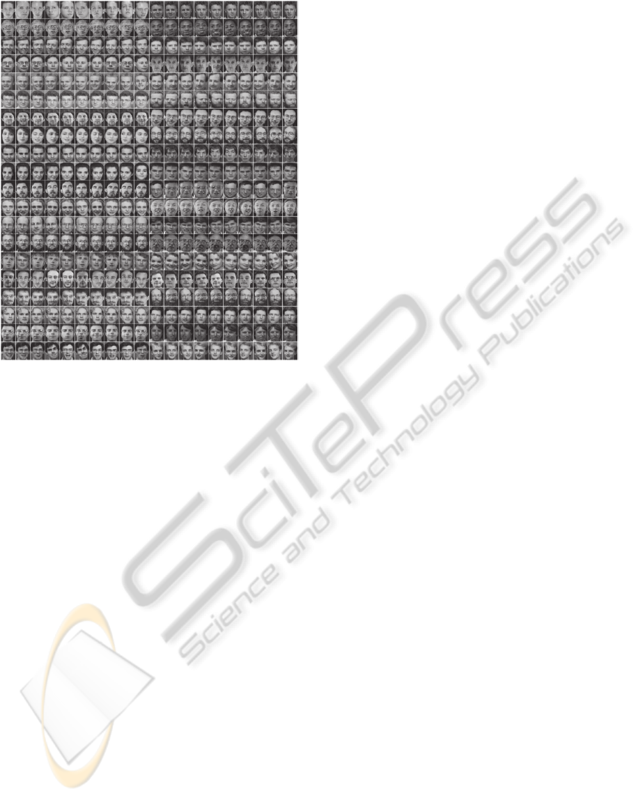
Figure 1: Data base ORL (Olivetti Research Laboratory).
This data base presents images with different
gestural positions, such as eyes open eyes close,
smile non-smile, glasses non-glasses and
illumination variations. The illumination variations
are not defined. All images are grey scale of 256
values, with an original size of 92 x 112 pixels.
3 EMPIRICAL MODE
DECOMPOSITION (EMD)
EMD algorithm is a method designed for multiscale
decomposition and time –frequency analysis, which
can analyze nonlinear and non-stationary data
(Huang et al., 1998).
With this method any time-series data set can be
decomposed into a finite and often small number of
Intrinsic Mode Functions (IMFs). These IMFs are
defined so as to exhibit locality in time and to
represent a single oscillatory mode. Each IMF
satisfies two basic conditions: (i) the number of
zero-crossings and the number of extrema must be
the same or differ at most by one in the whole
dataset, and (ii) at any point, the mean value of the
envelope defined by the local maxima and the
envelope defined by the local minima is zero (Huang
et al., 1998).
The EMD algorithm (Huang et al., 1998) for a
signal
can be summarized as follows.
(i) Determine the local maxima and minima of
;
(ii) Generate the upper and lower signal envelope
by connecting those local maxima and minima
respectively by an interpolation method;
(iii) Determine the local mean
, by averaging
the upper and lower signal envelope;
(iv) Subtract the local mean from the data:
.
(v) If
obeys the stopping criteria, then we
define
as an IMF, otherwise set
and repeat the process from step
(i).
Then, the empirical mode decomposition of a
signal
can be written as:
x
t
IMF
t
ε
t
(1)
Where n is the number of extracted IMFs, and the
final residue ε
t
is the mean trend or a constant.
4 MULTIVARIATE EMPIRICAL
MODE DECOMPOSITION
(MEMD)
EMD has achieved optimal results in data processing
(Diez et al., 2009); (Molla et al., 2010). However,
this method presents several shortcomings in
multichannel datasets. The IMFs from different time
series do not necessarily correspond to the same
frequency, and different time series may end up
having a different number of IMFs. For
computational purpose, it is difficult to match the
different obtained IMFs from different channels
(Mutlu and Aviyente, 2011).
To solve these shortcomings, an extension of
EMD to mEMD is required. In this approach the
local mean is computed by tanking an average of
upper and lower envelopes, which in turn are
obtained by interpolating between the local maxima
and minima. However, in general, for multivariate
signals, the local maxima and minima may not be
defined directly. To deal with these problems
multiple n-dimensional envelopes are generated by
taking signal projections along different direction in
n-dimensional spaces (Rehman and Mandic, 2010).
mEMD is the technique used in this paper to
compute all the decompositions.
The algorithm (Rehman and Mandic, 2010) can
be summarized as follows.
(i) Choose a suitable point set for sampling on an
BIOSIGNALS2013-InternationalConferenceonBio-inspiredSystemsandSignalProcessing
446

1
sphere (this
1
sphere resides in
an dimensional Euclidean coordinate system).
(ii) Calculate the projection, p
t
, of the
input signal v
t
along the direction vector,
x
for all k giving p
t
.
(iii) Find the time instants t
corresponding to the
maxima of the set of projected
signalsp
t
(iv) Interpolate t
,vt
to obtain multivariate
envelope curvese
t
.
(v) For a set of K direction vectors, the mean of the
envelope curves is calculated as
t
1K
⁄∑
e
t
(vi) Extract the detail
using
. If the detail
fulfills the stopping
criteria for a multivariate IMF, apply the above
procedure to
, otherwise apply it to
.
Then, the mEMD of a signal x
can be written as
detailed in equation 1.
5 NEURAL NETWORK
In recent years several classification systems have
been implemented using different techniques, such
as Neural Networks.
The widely used Neural Networks techniques are
very well known in pattern recognition applications.
An artificial neural network (ANN) is a
mathematical model that tries to simulate the
structure and/or functional aspects of biological
neural networks. It consists of an interconnected
group of artificial neurons and processes information
using a connectionist approach to computation. In
most cases an ANN is an adaptive system that
changes its structure based on external or internal
information that flows through the network during
the learning phase.
Neural networks are non-linear statistical data
modelling tools. They can be used to model complex
relationships between inputs and outputs or to find
patterns in data.
One of the simplest ANN is the so called
perceptron that consist of a simple layer that
establishes its correspondence with a rule of
discrimination between classes based on the linear
discriminator. However, it is possible to define
discriminations for non-linearly separable classes
using multilayer perceptrons (MLP).
The Multilayer Perceptron (Multilayer
Perceptron, MLP), also known as Backpropagation
Net (BPN), is one of the best known and used
artificial neural network model as pattern classifiers
and functions approximators (Lippman, 1987),
(Freeman and Skapura, 1991). It belongs to the so-
called feedforward networks class, and its topology
is composed by different fully interconnected layers
of neurons, where the information always flows
from the input layer, whose only role is to send input
data to the rest of the network, toward the output
layer, crossing all the existing layers (called hidden
layers) between the input and output. Essentially the
inner layers are responsible for carrying out
information processing, extracting features of the
input data.
Although there are many variants, usually each
neuron in one layer has directed connections to the
neurons of the subsequent layer but there is no
connection or interaction between neurons on the
same layer (Bishop, 1995, Hush and Horne, 1993).
6 IMAGE PROCESSING
The proposed procedure is detailed in Figure 2. The
system works as follow:
(i) The first 5 images are kept as representative for
each class. The mean image of these 5 images is
obtained for each class. These images will be
named as R
∀1 i N, where N is the total
number of classes.
(ii) The rest of the images will be used to be
classified as belonging to one of the classes.
(iii) For each new input image I to be classified,
mEMD decomposition between I and R
is
calculated, obtaining a total of N mEMD
decompositions:
D
mEMD(R
, I) ∀1
(2)
Each one of these D
decompositions is composed by
two sets (matrix) of IMFs, one set (matrix)
belonging to I and the other belonging to R
, and
each IMF have 986 points, where 986 is derived as
29*34 (unfolding an image to a vector, taking into
account that the original size of each image has
previously been reshaped to 29 x 34).
(iv) Then the distance between IMFs is calculated
for each D
i
, obtaining a vector of N values
corresponding to the distances between input
image I and each one of the classes.
EmpiricalModeDecomposition-basedFaceRecognitionSystem
447
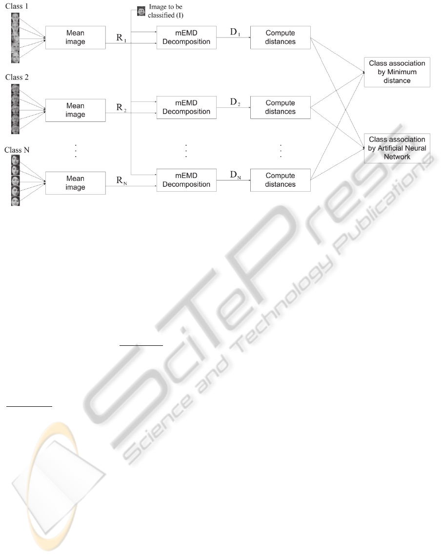
Figure 2: Scheme of the proposed image processing procedure.
Concerning distance measures, we have explored
different possibilities. Considering two matrix A and
B, corresponding to the obtained two sets (D
) of
IMFs, we can use:
1. Correlation coefficient between matrices A
and B
2. Matrix scalar product, also known as the
normalized Frobenius inner product:
,
:
‖
‖
‖
‖
(3)
Where A:B is the the Frobenius inner product of the
matrices A and B, defined as A:B traceA
B,
and
‖
‖
is the Frobenius norm defined as
‖
A
‖
traceA
A, where
T
denotes the transpose of a
matrix.
3. Frobenius norm of the differenceAB:
,
‖
‖
(4)
(v) The input image I is associated to a class as a
function of some criteria on the distance. For
that, two different methods were used. The first
one consist in associate the image to the
corresponding class obtained by the minimum
distance, therefore the decomposition D
i
that
presented the lowest distance value is associated
to that class. This is the same strategy
previously used in (Gallego-Jutglà and Solé-
Casals, 2012), but taking into account that now
the size of the images is greater, hence the
results are improved due to this fact. The second
one is based on an ANN classifier, where the
computed distances are used as input vector of
the system and the class association is done asw
a nonlinear mapping between vector distances
and classes.
For the classification step with ANN, a Multi
Layer Perceptrom (MLP) with one hidden layer of
100 neurons has been used. For the training and
validation phases, we used -fold cross-validation
with 10, in order to ensure solid results. In that
evaluation methodology the original sample set is
randomly divided into subsets. Then, a single
subset is retained as the validation data for testing
the model, and the remaining 1 subsets are used
as training data. The cross-validation process is
repeated times, with each of the subsets used
exactly once as the validation data. The obtained
results from the folds are then averaged in order to
produce a single estimation. The advantage of this
method is that all observations are used for both
training and validation, and each observation is used
for validation exactly once. This is the most robust
evaluation method because tries to overcome a
possible over-fitting. 10-fold cross-validation is
commonly used but in under-resourced condition the
leave-one-out cross-validation (LOOCV) could be
the best option. LOOCV uses a single observation
from the original set as the validation data, and the
remaining observations as the training data. This is
the same as a -fold cross-validation with equal to
the number of observations in the original sample
set. LOOCV is computationally expensive because it
requires many repetitions of training but
successfully with very small data sets.
BIOSIGNALS2013-InternationalConferenceonBio-inspiredSystemsandSignalProcessing
448
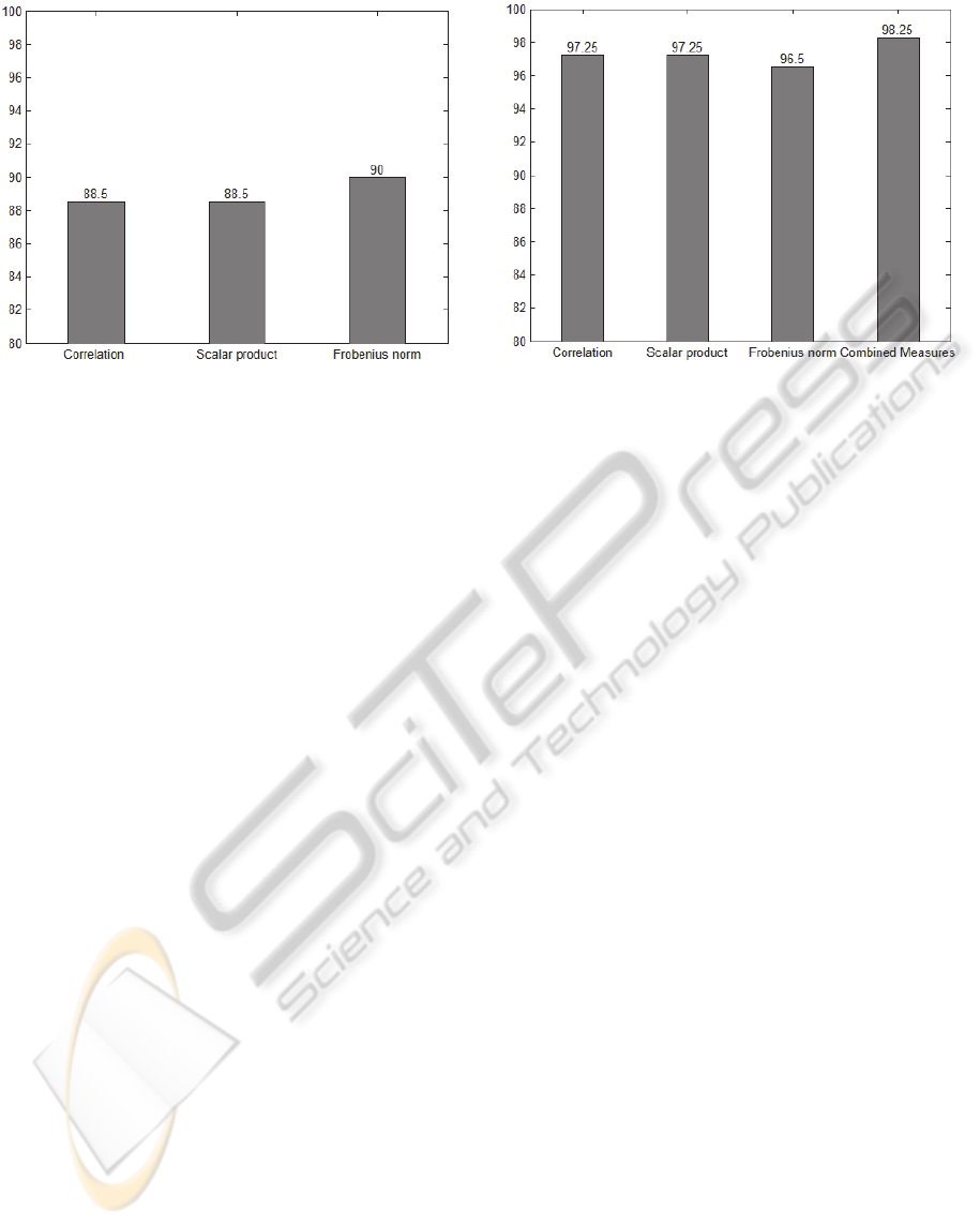
Figure 3: Obtained classification rates (%) for the three
different distances using the first method: class association
only based on the criterion of minimum distance. Exact
experimental values are presented at the top of each bar.
7 EXPERIMENTS
AND DISCUSSION
Initially, as explained in section 6, each image is
resized to 29 x 34. The choice of this size is justified
in order to have the same number of parameters (986
pixels) as in (Travieso et al., 2007), giving us the
possibility to compare performances.
Applying the detailed procedure to the images,
and using the described three different distances
measures, the following results are obtained:
Figure 3 summarize the obtained classification
results only based on the criterion of the minimum
distance. 88.5% of accuracy was obtained with
correlation and matrix scalar product, and a 90%
was obtained with Frobenius norm.
Figure 4 summarize the obtained classification
results using the MLP previously described. In that
figure, the results for the three distances (correlation,
scalar product and Frobenius) and for the
combination of the three distances are presented. In
this last case, the input vector of the MLP was
obtained concatenating all the three vector distances.
Classification rate obtained with MLP was much
better than before for the three distances: 97.25% for
correlation, 97.5% for scalar product and 96.5% for
Frobenius norm. The combination of all the three
distances increased this result up to a 98.25%.
As can be seen in Figure 3, the best result for the
first method is obtained with the 3
th
proposed
distance measure, the Frobenius norm distance.
Figure 4: Obtained classification rates (%) for the three
different distances and the combination of all of them,
using the second method: an ANN as a classifier. Exact
experimental values are presented at the top of each bar.
Contrarily, when we use ANN this measure is the
one with the lowest classification rate, even if the
difference is very small. By combining all the three
measures instead of only one measure, we obtain the
best results for the system (98.25%).
Comparing this result with results obtained in
(Travieso et al., 2007) we can see that we obtain the
same performance (98%).
In (Travieso et al., 2007) a DCT or DWT
(Biorthonal 4.4 family) parameterization was used
combined, with an SVM classifier. Here, the new
mEMD technique is used to decompose the data set
and the vector of distance measures is used as the
input to a MLP. Since our system do not use any
kind of transformation (DCT, DWT or others), a
combination of both strategies could even improve
the results and can be a future work to explore.
In any case, the method also needs to be tested
with other databases in order to ensure its general
performance.
Finally, some improvement of the computational
time would be interesting, as the mEMD algorithm
is not fast.
8 CONCLUSIONS
This study proposes a new strategy for face
recognition systems, where a new technique is used,
mEMD, and distance measures are used as input
vectors to an ANN in order to decide the class of the
input image.
With this technique, the simultaneously
decomposition of two images is computed, obtaining
EmpiricalModeDecomposition-basedFaceRecognitionSystem
449

the same number of IMF for both images. One
image is the image to be classified (input, unknown
image), and the other one is a reference image of one
class. This decomposition is performed with each
one of the reference image of each class. Once the
decompositions are computed, the distance between
the modes, arranged as a matrix, are computed. The
classification is done using two different methods. In
the first one the classification is only based on the
lowest distance between input image and reference
images decompositions, and in the other method the
classification uses these distances as input vector of
a MLP.
Three different distance measures were analyzed
and Frobenius norm distance measure gave the best
results when the association is based exclusively on
the distance. The combination of the three distances
gave the best result when an ANN was used as a
classifier.
The success of the proposed method is promising
and will encourage us to continuing investigating the
use of mEMD decomposition as a feature extracting
system for face recognition problems, with new and
bigger data base.
ACKNOWLEDGEMENTS
This work has been partially supported by the
University of Vic under the grant R904, and under a
predoctoral grant from the University of Vic to Mr.
Esteve Gallego-Jutglà, ("Amb el suport de l'ajut
predoctoral de la Universitat de Vic"); and by
SAIOTEK from the Basque Government, to Dra.
Karmele López-de-Ipiña.
REFERENCES
Bishop, C. M., (1995). Neural Networks for Pattern
Recognition. Oxford University Press.
Diez, P. F., Mut, V., Laciar, E., Torres, A., Avilla, E.
(2009). Application of the Empirical Mode
Decomposition to the Extraction of Features form
EEG signals for Mental Task Classification. 31
st
Annual International Conference of the IEEE EMBS.
Freeman, J. A., Skapura, D. M. (1991). Neural Networks:
Algorithms, Applications and Programming
Techniques. Addison-Wesley Publishing Company,
Inc. Reading, MA
Gallego-Jutglà, E., Solé-Casals, J., “Exploring mEMD for
face recognition”, BIOSIGNALS conference
proceedings, BIOSTEC 2012.
Huang, N. E., Shen, Z., Long,S. R., Wu, M. C., Shih, H.
H:, Zheng, Q., Yen, N. C., Tung, C. C., Liu, H. H.
(1998). The empirical mode decomposition and the
Hilbert spectrum for nonlinear and non-stationary time
series analysis. Proc. R. Soc. Lond., 495, 2317-2345.
Hush, D. R., Horne, B. G. (1993). Progress in supervised
neural networks. IEEE Signal Processing Magazine,10
(1), pp. 8-39.
Iancu, C., Corcoran, P., Costache, G. (2007). A Review of
Face Recognition Techniques for In-Camera
Applications. International Symposium on Signals,
Circuits and Systems,1,1-4.
Lippmann, D. E. (1987). An Introduction to Computing
with Neural Networks. IEEE ASSP Magazine, 3(4),
pp. 4-22
Molla, K. I., Tanaka, T., Rutkowski, T. M., Cichocki, A.,
(2010). Separation of EOG artifacts from EEG singals
using bivariate EMD. Acoustics Speech and Signal
Processing (ICASSP), 2010 IEEE Interational
Conference On. 562-565.
Mutlu, A. Y., Aviyente, S. (2011). Mutivariate Empirical
Mode Decomposition for Quantifying Multivariate
Phase Synchronization. EURASIP Jounal on Advances
in Signal Processing. Article ID 615717
Rehman, N., Mandic, D. P., (2010). Multivariate empirical
mode decomposition. Proc. R. Soc. A. 466, 1291-
1302.
Travieso, C. M., Solé-Casals, J., Zaiats, V., Alonso, J. B.,
Ferrer, M.A., “Reducción del Vector de Características
en Reconocimiento Facial”, XXIII Simposium
Nacional de la Unión Científica Internacional de
Radio URSI 2008.
Woodward, J. D., Orlans, N.M., Higgins P. T. (2003).
Biometrics. McGraw-Hill.
Xiao Q. (2007). Technology review - Biometrics-
Technology, Application, Challenge, and
Computational Intelligence Solutions. IEEE
Computational Intelligence Magazine, 2, 5-25.
BIOSIGNALS2013-InternationalConferenceonBio-inspiredSystemsandSignalProcessing
450
