
Learning Probabilistic Subsequential Transducers from Positive Data
Hasan Ibne Akram
1
and Colin de la Higuera
2
1
Technische Universit¨at M¨unchen, Munich, Germany
2
University of Nantes, Nantes, France
Keywords:
Probabilistic Transducers, Weighted Transducers, Transducer Learning, Grammatical Inference, Machine
Learning.
Abstract:
In this paper we present a novel algorithm for learning probabilistic subsequential transducers from a randomly
drawn sample. We formalize the properties of the training data that are sufficient conditions for the learning
algorithm to infer the correct machine. Finally, we report experimental evidences to backup the correctness of
our proposed algorithm.
1 INTRODUCTION
Probabilistic transducers or weighted transducers are
widely applied in the fields of natural language pro-
cessing, machine translation, bioinformatics, IT secu-
rity and many other areas. The generality of proba-
bilistic transducers allow them capturing other exist-
ing probabilistic models such as hidden Markov mod-
els (HMM) (Rabiner, 1990) or pair hidden Markov
models (PHMM) (Durbin et al., 1998). Due to
the widespread use and applicability of probabilistic
transducers, the learnability issue of such models is
an important problem.
Probabilistic subsequential transducers (PSTs) are
deterministic finite state machines w.r.t. the input
symbols, i.e., there can be no two outgoing edges
from a given state with same input label having dif-
ferent output labels and/or different destination states.
Due to its deterministic property, PSTs have less ex-
pressive power than PHMM and probabilistic trans-
ducers in general. Despite of the low expressive
power of PSTs, the computational complexity (e.g.,
translation of a given string, computing the probabil-
ity of a translation pair) is linear w.r.t. the size of the
input string. Therefore, there is an interesting trade-
off between PHMM or probabilistic transducers and
PSTs in terms of expressive power and computational
complexity.
The problem of learning PSTs in an identification
of the limit model has been investigated by Akram
et al. in (2012), where they have proposed the al-
gorithm APTI (Algorithm for Learning Probabilistic
Transducers). APTI uses a combination of state merg-
ing approach and probabilistic queries to infer the tar-
get machine.
In this paper we propose a novel algorithm
(APTI2) for learning PSTs that learns from an em-
pirical distribution of positive examples. The main
idea of our proposed algorithm is inspired by previous
work in subsequential transducer learning (Oncina
and Garc´ıa, 1991; Oncina et al., 1993) and probabilis-
tic finite automata (PFA) learning such as (Carrasco
and Oncina, 1994; Thollard et al., 2000; Carrasco and
Oncina, 1999).
This paper aims to utilize the lessons learnt from
subsequential transducer learning and PFA learning
and attempts to solve the problem of learning PSTs
from positive examples.
The fact that APTI2 makes no use of an oracle,
makes it usable in practice. We present an analysis of
the algorithm to illustrate the theoretical boundaries.
Finally, we present experimental results based on ar-
tificially generated datasets.
2 DEFINITIONS AND
NOTATIONS
Let [n] denote the set {1,...,n} for each n ∈ N. An al-
phabet Σ is a non-empty set of symbols and the sym-
bols are called letters. Σ
∗
is a free-monoid over Σ.
Subsets of Σ
∗
are known as (formal) languages over
Σ. A string w over Σ is a finite sequence w = a
1
... a
n
of letters. Let |w| denote the length of the string w.
In this case we have |w| = |a
1
... a
n
| = n. The empty
479
Ibne Akram H. and de la Higuera C..
Learning Probabilistic Subsequential Transducers from Positive Data.
DOI: 10.5220/0004359904790486
In Proceedings of the 5th International Conference on Agents and Artificial Intelligence (LAFLang-2013), pages 479-486
ISBN: 978-989-8565-38-9
Copyright
c
2013 SCITEPRESS (Science and Technology Publications, Lda.)

string is denoted by ε. For every w
1
,w
2
∈ Σ
∗
, w
1
· w
2
is the concatenation of w
1
and w
2
. The concatenation
of ε and a string w is given by ε· w = w and w· ε = w.
When decomposing a string into substrings, we will
write w = w
1
,.. . ,w
n
where ∀i ∈ [n],w
i
∈ Σ
∗
. If w =
w
1
w
2
is a string, then w
1
is a prefix. Given a language
L ⊆ Σ
∗
, the prefix set of L is defined as Pref(L ) =
{u ∈ Σ
∗
: ∃v ∈ Σ
∗
,uv ∈ L }. Pref(w) is defined as the
set of all the substrings of w that are prefixes of w.
The longest common prefix of L is denoted as lcp(L ),
where lcp(L ) = w ⇐⇒ w ∈
T
x∈L
Pref(x) ∧ ∀w
′
∈
T
x∈L
Pref(x) ⇒ |w
′
| ≤ |w|. Less formally, lcp is a
function that returns the longest possible string which
is the prefix of all the strings in a given set of strings.
For example, for L = {aabb,aab, aababa,aaa} the
lcp(L ) is aa.
2.1 Stochastic Transductions
In order to represent transductions we now use two
alphabets, not necessarily distinct, Σ and Ω. We use
Σ to denote the input alphabet and Ω to denote the
output alphabet. For technical reasons, to denote the
end of an input string we use a special symbol ♯ as an
end marker.
A stochastic transduction R is given by a function
Pr
R
: Σ
∗
♯ × Ω
∗
→ R
+
, such that :
∑
u∈Σ
∗
♯
∑
v∈Ω
∗
Pr
R
(u,v) = 1,
where Pr
R
(u,v) is the joint probability of u and
v. Otherwise stated, a stochastic transduction R is
the joint distribution over Σ
∗
♯ × Ω
∗
. Let L ⊂ Σ
∗
♯ and
L
′
⊂ Ω
∗
;
Pr
R
(L ,L
′
) =
∑
u∈L
∑
v∈L
′
Pr
R
(u,v).
Example 1. The transduction R : Σ
∗
♯ × Ω
∗
→ R
+
where Pr
R
(a
n
♯,1
n
) =
1
2
n
,∀n > 0, and Pr
R
(u,v) = 0
for every other pair.
In the sequel, we will use R to denote a stochastic
transduction and T to denote a transducer. Note that
the end marker ♯ is needed for technical reasons only.
The probability of generating a ♯ symbol is equivalent
to the stopping probability of an input string.
2.2 Probabilistic Subsequential
Transducers
A transduction scheme can be modeled by transduc-
ers or probabilistic transducers. In this section, we
will define probabilistic subsequential transducers
(PST) that can be used to model a specific subclass
of stochastic transductions.
Definition 1. A probabilistic subsequential trans-
ducer (PST) defined over the probability semiring R
+
is a 5-tuple T = hQ,Σ∪ {♯},Ω,{q
0
},Ei where:
• Q is a non-empty finite set of states,
• q
0
∈ Q is the unique initial state,
• Σ and Ω are the sets of input and output alphabets,
• E ⊆ Q × Σ ∪ {♯} × Ω
∗
× R
+
× Q, and given e =
(q,a,v,α,q
′
) we denote: prev[e] = q, next [e] =
q
′
, i[e] = a, o[e] = v, and prob[e] = α,
• the following conditions hold:
– ∀q ∈ Q,
∀(q,a,v,α,q
′
),(q,a
′
,v
′
,β,q
′′
) ∈ E, a = a
′
⇒
v = v
′
, α = β, q
′
= q
′′
,
– ∀q ∈ Q,
∑
a∈Σ∪{♯},q
′
∈Q
Pr(q,a,q
′
) = 1,
– ∀(q,a,v,α,q
′
) ∈ E, a = ♯ ⇒ q
′
= q
0
.
3 THE LEARNING SAMPLE
When learning, the algorithm will be given a ran-
domly drawn sample: the pairs of strings will be
drawn following the joint distribution defined by the
target PST. Therefore, such a sample is a multiset,
since more frequent translation pairs may occur more
than once and is called a learning sample. The formal
definition of a learning sample is the following:
Definition 2. A learning sample is a multiset
S
n
hX, fi where X = {(u,v) : u ∈ Σ
∗
♯,v ∈ Ω
∗
}, f :
(u,v) → [n], and f(u,v) is the multiplicity or number
of occurrence of (u,v) in X.
For simplicity, for a given S
n
hX, f i, if (u♯,v) ∈ X,
we will write (u♯,v) ∈ S
n
unless the context requires
to be more specific. We assume that the learning sam-
ple obeys the following property: ∀(u♯,v),(u♯, v
′
) ∈
S
n
⇒ v = v
′
, i.e., the translation pairs are un-
ambiguous.
4 FREQUENCY TRANSDUCERS
In our proposed solution, the learner utilizes the rela-
tive frequency of the observed data. It starts by build-
ing a tree like transducer that incorporates the fre-
quencies of the training data and is an exact represen-
tation of the training data. In the next phase of the
algorithm, the learner makes iterative state merges.
The merge acceptance decision is based on the consis-
tency of translation w.r.t. the training data and statis-
tical test using the relative frequencies. At this point
ICAART2013-InternationalConferenceonAgentsandArtificialIntelligence
480

we will define a new type of transducer that incorpo-
rates the frequencies of translations, called frequency
subsequential transducer.
Definition 3 (Frequency Finite Subsequential Trans-
ducer). A frequency finite subsequential transducer
(FFST) is a 6-tuple T = hQ,Σ ∪ {♯},Ω,{q
0
},E,F
r
i
where ψ(T) = hQ,Σ∪ {♯},Ω,{q
0
},Ei is an ST and F
r
is the frequency function defined as F
r
: e → N, where
e ∈ E.
An FFST is well defined or consistent if the fol-
lowing property holds:
∀q ∈ Q\{q
0
},
∑
e∈E:next[e]=q
F
r
(e) =
∑
e∈E[q]
F
r
(e) (1)
Since q
0
is the only initial state, the sum of the fre-
quencies of the outgoing edges is assumed to be num-
ber of frequency entering the initial state, and there-
fore q
0
is treated specifically. Figure 1(a) depicts an
example of a consistent FFST.
Intuitively,an FFST is an object where the weights
are the frequencies of the transitions instead of proba-
bilities. F
r
(e) = n should be interpreted as: the edge e
is used n times. FFSTs can be converted to equivalent
PSTs.
Next we define a prefix tree transducer that is an
exact representation of the observed sample S
n
and
holds the frequencies of the strings.
Definition 4 (Frequency Prefix Tree Subsequen-
tial Transducer). A frequency prefix tree subse-
quential transducer (FPTST) is a 6-tuple T =
hQ,Σ∪ {♯},Ω,{q
0
},E,F
r
i where ψ(T) =
hQ,Σ∪ {♯},Ω,{q
0
},E,F
r
i is an FFST and T is
built from a training sample S
n
such that:
• Q =
[
(u,v)∈S
n
{q
x
: x ∈ Pref(u)},
• E = {e | prev[e] = q
u
,next [e] = q
v
⇒ v = ua, a ∈
Σ,i[e] = a,o[e] = ε},
• ∀q
u
∈ Q,∀e ∈ E [q] , i[e] = ♯,o[e] = v if (u,v) ∈
S
n
,⊥ otherwise,
• ∀e ∈ E [q
0
],F
r
(e) =
|{a : i[e] = a,a ∈ Pref({u : (u,v) ∈ S
n
})}|,
• ∀q
u
∈ Q \ {q
0
},∀e ∈ E [q
u
], F
r
(e) =
|{a : ua ∈ Pref({x : (x,y) ∈ S
n
})}|.
An FPTST is said to be in an onward form if the
following condition holds:
∀q ∈ Q\{q
0
},lcp
[
e∈E[q]
{o[e]}
!
= ε.
An FPTST is essentially an exact representation
of the training data augmented with the observed fre-
quencies of the training data. The frequencies can be
utilized to make statistical tests: relative frequencies
can be compared by means of Hoeffding tests (Ho-
effding, 1963) during the state merging phase of the
algorithm.
Let f
1
, n
1
and f
2
, n
2
be two pairs of observed fre-
quencies of symbols and number of trials respectively.
f
1
n
1
−
f
2
n
2
<
r
1
2
1
n
1
+
1
n
2
log
2
δ
. (2)
It is noteworthy that the Hoeffding bound is rela-
tively weak or bad approximation and there are bet-
ter alternatives. However, to demonstrate the proof of
concept in our algorithm we will only use the Hoeffd-
ing bound.
5 THE ALGORITHM
The proposed algorithm APTI2 executes in three
phases: initialization, state merging and conversion
of the inferred FFST to an equivalent PST. In the ini-
tialization phase, the algorithm builds an FPTST in an
onward form, from the learning sample S
n
. This is
achieved by the routine ONWARDFPTST (Algorithm
1, line 1). Next, the state merging phase of APTI2
begins and is similar to the OSTIA algorithm, with a
modified state merging strategy. The details of OSTIA
can be found in (Oncina et al., 1993; Castellanos
et al., 1998; de la Higuera, 2010). Here we follow the
recursive formalism given in (de la Higuera, 2010).
The algorithm APTI2 (Algorithm 1) selects a candi-
date pair of RED and BLUE states in lex-length order
using the CHOOSE
<
lex
function. The MERGE func-
tion merges the two selected states and recursively
performs a cascade of folding of a number of edges
(see (de la Higuera, 2010) for details). As a result
of the onwarding process, some of the output strings
may come too close to the initial state. During the run
of the algorithm these strings or the suffixes of these
strings are pushed back in order to make state merg-
ing possible by deferring the translations; this is done
in the standard way as in OSTIA. During the recursive
fold operation, it is actually decided whether a merge
is accepted or not. The algorithm APTI2 employs the
following condition for a merge to be accepted:
• ∀e
b
∈ E [q
b
],∀e
r
∈ E [q
r
],i[e
b
] = i[e
r
] ⇒
1. o[e
b
] = o[e
r
],
2. inequality (2) holds for f
1
= F
r
(e
b
),
n
1
=
∑
e∈E[q
b
]
F
r
(e) and f
2
= F
r
(e
r
),
n
2
=
∑
e∈E[q
r
]
F
r
(e).
Condition 1 is essentially similar to the one used in
OSTIA. The second condition is to check whether
the relative frequencies related to two states are close
LearningProbabilisticSubsequentialTransducersfromPositiveData
481

q
0
q
1
q
2
♯ : ε(60)
a : x(50)
b : y(35)
a : xx(30)
a : x(5)
♯ : x(20)
b : y(65)
b : y(15)
(a)
q
0
q
1
q
2
♯ : ε(0.41)
a : x(0.35)
b : y(0.24)
a : xx(0.32)
a : x(0.13)
♯ : x(0.5)
b : y(0.68)
b : y(0.37)
(b)
Figure 1: Figure 1(a) shows an example of an FFST. Figure 1(b) shows an equivalent PST of the FFST shown in Figure 1(a).
Notice that the FFST in Figure 1(a) is consistent as per condition (1).
enough. In this case the Hoeffding bound is used
as a statistical test. The state merging phase termi-
nates whenever there are no more BLUE states to be
merged. Finally, in the third phase, the inferred FFST
is converted to an equivalent PST using the hypotheti-
cal routine CONVERTFFSTTOPST (Algorithm 1, line
13)
Algorithm 1: APTI2.
Input: a sample S
n
Output: a PST T
1 T ← ONWARDFPTST(S
n
);
2 RED ← {q
ε
};
3 BLUE ← {q
a
: a ∈ Σ ∩ Pref({u : (u, v) ∈ S
n
)})};
4 while BLUE 6=
/
0 do
5 q = CHOOSE
<
lex
(BLUE);
6 for p ∈ RED in lex-length order do
7 (T
′
,IsAccept) ← MERGE(T, p, q);
8 if IsAccept then
9 T ← T
′
;
10 else
11 RED ← RED ∪ {q};
12
BLUE ← {q: ∀p ∈ RED,∀e ∈ E [p] ,
q = next[e] ∧ q /∈ RED};
13 CONVERTFFSTTOPST(T);
14 return T;
6 ANALYSIS OF THE
ALGORITHM
We recall the definition of a learning sample S
n
hX, fi
where the frequency of a translation pair (u,v)
is given by f(u,v). Similarly, we define the
prefix frequency F
S
n
w.r.t. a learning sam-
ple S
n
as the following: F
S
n
(uΣ
∗
,v) =
|{(w, x) : (w,x) ∈ S
n
∧ u ∈ Pref(w)}|. Less for-
mally, F
S
n
(uΣ
∗
,v) is the number of translation pairs
where the input string starts with the substring u.
We define the prefix set (PR) and the short pre-
fix set (SP) with respect to a stochastic transduction
R as the following: PR(R ) = {u ∈ Σ
∗
|(u,v)
−1
R 6=
/
0,v ∈ Ω
∗
} and SP(R ) = {u ∈ PR(R )|(u,v)
−1
R =
(w, x)
−1
R ⇒ |u| ≤ |w|}. The kernel set (K) of R is
defined as follows: K(R ) = {ε} ∪ {ua ∈ PR(R )|u ∈
SP(R ) ∧ a ∈ Σ}. Note that SP is included in K.
We use the above definitions to define the suffi-
cient conditions a learning sample must obey in order
to obtain a correct PST. The sufficient condition for a
learning sample S
n
hX, fi in order to learn the syntac-
tic machine w.r.t. an SDRT R are the following:
1. ∀u ∈ K,∃(uw, vx) ∈ X such that w ∈ Σ
∗
,vx ∈
Ω
∗
,(w,x) ∈ (u, v)
−1
R ,
2. ∀u ∈ SP, u
′
∈ K, if (u,v)
−1
R 6= (u
′
,v
′
)
−1
R where
v,v
′
∈ Ω
∗
, then any one of the following holds:
(a) ∃(uw,vx),(u
′
w, v
′
x
′
),(ur,vy),(u
′
r,v
′
y
′
) ∈ X
such that for a given value of δ:
f(uw,vx)− f (ur,vy)
F
S
n
(uΣ
∗
,z)
−
f(u
′
w,v
′
x
′
)− f(u
′
r,v
′
y
′
)
F
S
n
(u
′
Σ
∗
,z
′
)
<
r
1
2
log
2
δ
1
F
S
n
(uΣ
∗
,z)
+
1
F
S
n
(u
′
Σ
∗
,z
′
)
(b) ∃(uw,vx),(u
′
w, v
′
x
′
),∈ X such
that: (w, x) ∈ (u, v)
−1
R ,(w,x
′
) ∈
(u
′
,v
′
)
−1
R ,x 6= x
′
3. ∀u ∈ K,∃(uw,vx)(uw
′
,vx
′
) ∈ X such that
lcp(x,x
′
) = ε ∧ w 6= w
′
.
With the conditions above, the properties of a
learning sample S
n
have been formalized in order to
guarantee the algorithm to learn correctly. The con-
dition 1, 2(b), and 3 are essentially similar to its non-
probabilistic counterpart OSTIA (Oncina et al., 1993).
Condition 1 is to ensure that there are at least as many
states in the learning phase as the target transducer.
Condition 2(b) is for making merge decisions w.r.t.
the output strings. Condition 3 ascertains the align-
ments of the output strings by factorizing them during
ICAART2013-InternationalConferenceonAgentsandArtificialIntelligence
482

the state merging phase. Condition 2(b) is not guaran-
teed if the transduction scheme is not a total function
(Oncina et al., 1993), i.e., it is not sufficient to make
the merge decision if the transduction scheme is a par-
tial function. In order to overcome this issue, in our
proposed algorithm we have used the frequencies of
the given data. Condition 2(a) ensures that the rela-
tive frequencies of the observed data is sufficient to
distinguish non-mergable states by means of Hoeffd-
ing bound. The inequality shown in condition 2(a) is
from inequality 2.
Notice that condition 2(a) depends on the value of
δ. Carrasco and Oncina have discussed how a large
or a small value of δ affects the merge decision in
(Carrasco and Oncina, 1994). Basically, if the size
of the learning sample S
n
is significantly large, one
could keep δ negligibly small. On the contrary, for a
relatively small size of learning sample S
n
, δ requires
to be sufficiently high.
The runtime complexity of algorithm APTI2
is given by O ((kS
n
k)
3
(m + n) + kS
n
kmn), where:
kS
n
k =
∑
(u,v)∈S
n
|u| and m = max{|u| : (u,v) ∈ S
n
}.
The FPTST can be built in linear time w.r.t. kS
n
k.
We will now analyze the outermost while loop in the
APTI2 algorithm. Being pessimistic, there will be at
most kS
n
k numberof states in the FPTST. In the worse
case, if no merges are accepted, there will be O (kS
n
k)
executions of the outermost while loop and O (kS
n
k
2
)
executions of the inner for loop, resulting O (kS
n
k
3
)
executions of the core algorithm. In each of these ex-
ecutions, lcp operation can be implemented in O (m)
times and the pushback operation in O (n) times. As-
suming that all arithmetic operations are computed
in unit time, the total core operation of APTI2 can
be bounded by O ((kS
n
k)
3
(m + n) + kS
n
kmn). This
runtime complexity is pessimistic and the runtime of
APTI2 is much lower in practice. Experimental ev-
idence of runtime of APTI2 is presented in the next
section.
7 EXPERIMENTAL RESULTS
We conduct our experiments with two types of data
sets: 1) artificial data sets generated from random
transducers 2) data generated from the Miniature Lan-
guage Acquisition (MLA) task (Feldman et al., 1990)
adapted to English-French translations.
For the artificial data sets, we first generate a ran-
dom PST with m states. The states are numbered
from q
0
to q
m−1
where state q
0
is the initial state.
The states are connected randomly; labels on transi-
tions preserve the deterministic property. Then the
unreachable states are removed. The outputs are as-
signed as random strings drawn from a uniform dis-
tribution over Ω
≤k
, for an arbitrary value of k. The
probabilities of the edges are randomly assigned mak-
ing sure the following condition holds:
∀q
i
∈ Q,
∑
e∈E[q
i
]
prob[e] = 1 (3)
Using the target PST, the training sample is gen-
erated following the paths of the PST. The test data is
also generated in the similar manner. In order to test
the algorithm with unseen examples, we make sure
that the test set and the training set are disjoint.
As a measure of correctness we compute two met-
rics: word error rate (WER) and sentence error rate
(SER). Intuitively, WER is the percentage of sym-
bol errors in the hypothesis translation w.r.t. the ref-
erence translation. For each test pair, the Levenshtein
distance (Levenshtein, 1966) between the reference
translation and hypothesis translation is computed
and divided by the length of the reference string. The
mean of the scores computed for each test pair is re-
ported as the WER. On the other hand the SER is
more strict; it is the percentage of wrong hypothesis
translations w.r.t. the reference translations.
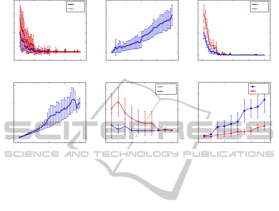
The objectives of the first experiment (see Fig-
ure 2(a) and Figure 2(b)) are to demonstrate the cor-
rectness of our algorithm and to study the practical
runtime. Figure 2(a) shows experiments conducted
on randomly generated PSTs with 5 states and |Σ| =
|Ω| = 2. We start with a training sample size 200,
we keep incrementing the training size by 200 up to a
size of 20000. For every training size the experiment
is repeated 10 times by generating new datasets. The
mean of these 10 experimental results is reported. We
have conducted the experiment for 10 random PSTs.
Thus, in total we have conducted 10000 trials. Fig-
ure 2(a) shows the mean of the results obtained from
10 random PSTs. As the Figure 2(a) shows, the error
rate is approaching zero. As expected, the WER in
most cases remains below SER. The execution time
for this experiment is reported in Figure 2(b). The
results of this experiment tell us that APTI2 shows ac-
ceptable error rate with 5000 training examples, and
from a training size of 10000 the error rate is close to
zero. The runtime in practice is much lower than the
theoratical bound and almost linear.
In our second experiment (Figures 2(c) and 2(d)),
we aim to learn slightly larger PSTs. In this second
experiment we have taken a randomly generated PSTs
with 10 states and |Σ| = |Ω| = 2. We start with a train-
ing sample size 1000, we keep incrementing the train-
ing size by 1000 up to a size of 40000. Similar to the
previous experiment, experiments with each training
sample size are repeated 10 times. The experiment is
conducted for 10 random PSTs. The results of this ex-
LearningProbabilisticSubsequentialTransducersfromPositiveData
483
0
0.5
1
1.5
2
·10
4
0
0.2
0.4
0.6
0.8
1
Size of the learning sample (S
n
)
Error rate
WER
SER
(a)
0
0.5
1
1.5
2
·10
4
0
20
40
Size of the learning sample (S
n
)
Time in seconds
(b)
0 1 2 3 4
·10
4
0
0.2
0.4
0.6
0.8
Size of the learning sample (S
n
)
Error rate
WER
SER
(c)
0 1 2 3 4
·10
4
0
100
200
300
Size of the learning sample (S
n
)
Time in seconds
(d)
0.2 0.4
0.6
0.8 1
·10
4
0
0.5
1
Size of the learning sample (S
n
)
Error rate
APTI2
OSTIA
(e)
0.2 0.4
0.6
0.8 1
·10
4
0
10
20
30
40
50
Size of the learning sample (S
n
)
Time (second)
APTI2
OSTIA
(f)
Figure 2: Performance of APTI2 reported for the artificially generated data set (Figures 2(a), 2(b), 2(c), and 2(d)) and the data
set for the MLA task (Figures 2(e), 2(f)).
periment show us APTI2 requires larger size of learn-
ing sample when the number of states of the target
machine is bigger and again, the execution time re-
mains reasonable. However, a target size of 10 is still
not large enough for many practical tasks.
Finally, we have conducted another experiment
with the Feldman dataset. The target PST consists of
22 states. The objectives of this experiment were to
make a comparison of prediction accuracy and of run-
time for OSTIA and APTI2. Here we start with 1000
training pairs and incremented by 1000 till obtaining
10000 training pairs. Each data point is repeated 10
times for statistical significance. The results are de-
picted in Figure 2(e) and 2(f). The results of Figure
2(e) demonstrate significant improvement in predic-
tion accuracy of APTI2 in comparison with OSTIA.
APTI2 attains almost perfect accuracy with only 4000
training examples while OSTIA continues to make an
error of about 30%. As we increase the number of
training data, at one point, when the number of train-
ing examples is about 8000, OSTIA also performs as
well as APTI2. However, APTI2 attains this accuracy
rate with only half of the number of training exam-
ples. Figure 2(f) shows that the execution time of
APTI2 is higher than that of OSTIA, yet it always re-
mains reasonable (below 40 seconds).
We have implemented APTI2 using an open
source C++ library for weighted transducers (Al-
lauzen et al., 2007). Figures 2(b), 2(d), and 2(f) show
the execution times for APTI2 using our implemen-
tation. Although, the theoretical worst case runtime
complexity of APTI2 is cubic, in practice APTI2 ex-
hibits much lower execution time.
8 CONCLUSIONS
We have presented a learning algorithm APTI2 that
learns any PST provided a characteristic training sam-
ple is given. We have also presented experimental re-
sults based on synthetic data to proof the correctness
of our algorithm. Moreover, based on our implemen-
tation, we have reported that the runtime complexity
of APTI2 in practice is much lower than the theoreti-
cal worst case runtime complexity.
The limitation of our work is twofold: first, our
model is restricted to regular stochastic bi-grammar,
and hence not capable of capturing many practical
scenarios, e.g., natural languages. Second, as a statis-
tical test we have used a basic Hoeffding bound. We
believe that more sophisticated statistical tests will
lead to better accuracy of the algorithm.
ICAART2013-InternationalConferenceonAgentsandArtificialIntelligence
484

REFERENCES
Akram, H. I., de la Higuera, C., and Eckert, C. (2012).
Actively learning probabilistic subsequential trans-
ducers. In Proceedings of ICGI, volume 21 of
JMLR:Workshop and Conference Proceedings. MIT
Press.
Allauzen, C., Riley, M., Schalkwyk, J., Skut, W., and
Mohri, M. (2007). Openfst: A general and efficient
weighted finite-state transducer library. In Proceed-
ings of CIAA, volume 4783 of Lecture Notes in Com-
puter Science, pages 11–23. Springer.
Carrasco, R. C. and Oncina, J. (1994). Learning stochas-
tic regular grammars by means of a state merging
method. In Proceedings of ICGI, volume 862 of
Lecture Notes in Computer Science, pages 139–152.
Springer.
Carrasco, R. C. and Oncina, J. (1999). Learning determinis-
tic regular grammars from stochastic samples in poly-
nomial time. Rairo - Theoratical Informatics and Ap-
plications, 33(1):1–20.
Castellanos, A., Vidal, E., Var´o, M. A., and Oncina, J.
(1998). Language understanding and subsequential
transducer learning. Computer Speech & Language,
12(3):193–228.
de la Higuera, C. (2010). Grammatical Inference: Learn-
ing Automata and Grammars. Cambridge University
Press.
Durbin, R., Eddy, S. R., Krogh, A., and Mitchison, G.
(1998). Biological Sequence Analysis: Probabilistic
Models of Proteins and Nucleic Acids. Cambridge
University Press.
Feldman, J. A., Lakoff, G., Stolcke, A., and Weber, S. H.
(1990). Miniature language acquisition: A touch-
stone for cognitive science. Technical Report TR-90-
009, International Computer Science Institute, Berke-
ley CA.
Hoeffding, W. (1963). Probability inequalities for sums of
bounded random variables. American Statistical As-
sociation Journal, 58:13–30.
Levenshtein, V. I. (1966). Binary codes capable of correct-
ing deletions, insertions and reversals. Soviet Physics
Doklady, 10:707.
Oncina, J. and Garc´ıa, P. (1991). Inductive learning
of subsequential functions. Technical report, Univ.
Polit’ecnica de Valencia.
Oncina, J., Garc´ıa, P., and Vidal, E. (1993). Learning subse-
quential transducers for pattern recognition interpre-
tation tasks. IEEE Trans. Pattern Anal. Mach. Intell.,
15(5):448–458.
Rabiner, L. R. (1990). Readings in speech recognition.
chapter A tutorial on hidden Markov models and se-
lected applications in speech recognition, pages 267–
296. Morgan Kaufmann Publishers Inc.
Thollard, F., Dupont, P., and de la Higuera, C. (2000). Prob-
abilistic dfa inference using Kullback-Leibler diver-
gence and minimality. In Proceedings of ICML, pages
975–982. Morgan Kaufmann.
APPENDIX
An Example Run of the APTI2 Algorithm
As an example of a stochastic regular bi-language, let
us consider the following:
Example 2. The transduction R : Σ
∗
♯ × Ω
∗
→ R
+
where Pr
R
(a
n
ba
m
♯,x
n
yx
m
) =
1
2(3
n
4
m
)
,∀n,m ≥ 0. and
Pr
R
(u,v) = 0 for every other pairs.
Figure 3 shows the PST in the onward and min-
imal form (for details about the minimal form see
(Akram et al., 2012)) that generates R . We will con-
sider the PST shown in Figure 3 as the target PST. The
training data w.r.t. the target PST (Figure 3) is given
in Table 1.
q
0
q
1
b : y(
2
3
)
♯ : ε(
3
4
)
a : x(
1
3
) a : x(
1
4
)
Figure 3: The PST in canonical normal form that generates
R defined in Example 2.
Table 1: Training data for the target PST in Figure 3.
input output frequency
b♯ y 500
ab♯ xy 160
ba♯ x 120
aab♯ xxy 50
aba♯ xyx 40
total 870
Next, an onward FPTST is built from the data
given in Table 1. The FPTST is shown in Figure 4.
The states q
0
is initiated as a RED state and states q
1
and q
2
are initiated as BLUE states. Here for the Ho-
effding bound test, the value of δ is set arbitrarily to
0.5.
The first merge candidate pair of states are q
0
and
q
1
. The merge between them is accepted and the re-
sulting transducer is shown in Figure 5.
Next, the algorithm tries to merge q
0
and q
0
(Fig-
ure 6). This merge is rejected because the Hoeffding
bound test (Equation 2) returns false. The state q
2
is
promoted to RED and consequently the states q
5
and
q
6
are added as RED states (Figure 7).
Then the Algorithm tries to merge the states q
0
and q
5
which is also rejected because the Equation 2
returns false. Now the next candidate merge pair is q
2
and q
5
. This merge is accepted (Figure 8).
LearningProbabilisticSubsequentialTransducersfromPositiveData
485

The next candidate pair of merge is q
0
and q
6
which is accepted and the resulting transducer is de-
picted in Figure 9.
Finally, the FFST is converted into a PST (Figure
10) and the algorithm terminates. The inferred PST is
shown in Figure 10.
q
2
q
4
q
0
q
1
q
3
q
6
q
8
q
7
q
5
q
9
q
10
q
11
q
12
a : x(250)
b : y(620)
a : xy(50)
b : y(200)
a : ε(120)
♯ : ε(500)
b : ε(50) ♯ : ε(50)
a : x(40)
♯ : ε(160)
♯ : ε(40)
♯ : ε(120)
Figure 4: An onward F
PTST built from stochastic sample
given in Table 1.
q
2
q
0
q
6
q
5
q
10
a : x(300)
b : y(870)
a : ε(160)
♯ : ε(710)
♯ : ε(160)
Figure 5: After merging and folding q
0
and q
1
.
q
2
q
0
q
6
q
5
q
10
a : x(300)
b : y(870)
a : ε(160)
♯ : ε(710)
♯ : ε(160)
Figure 6: Merge between q
0
and q
2
is rejected.
q
2
q
0
q
6
q
5
q
10
a : x(300)
b : y(870)
a : ε(160)
♯ : ε(710)
♯ : ε(160)
Figure 7: q
2
is promoted to RED and as a consequence of
that q
5
and q
6
are added to BLUE.
q
2
q
0
q
6
a : x(300)
b : y(870)
a : ε(160)
♯ : ε(870)
Figure 8: After merging and folding q
2
and q
5
.
q
2
q
0
a : x(300)
b : y(870)
a : ε(160)
♯ : ε(870)
Figure 9: After merging and folding q
0
and q
6
.
q
2
q
0
a : x(0.26)
b : y(0.74)
a : ε(0.16)
♯ : ε(0.84)
Figure 10: After converting the FFST shown in Figure 7 to
a PST.
ICAART2013-InternationalConferenceonAgentsandArtificialIntelligence
486
