
Analysis Cloud
Running Sensor Data Analysis Programs on a Cloud Computing Infrastructure
Jan Sipke van der Veen
1
, Bram van der Waaij
1
, Matthijs Vonder
1
, Marc de Jonge
1
,
Elena Lazovik
1
and Robert J. Meijer
1,2
1
TNO, Groningen, The Netherlands
2
University of Amsterdam, Amsterdam, The Netherlands
K
eywords:
Data Analysis, Data Science, Sensor Data, Cloud Computing.
Abstract:
Sensors have been used for many years to gather information about their environment. The number of sensors
connected to the internet is increasing, which has led to a growing demand of data transport and storage
capacity. In addition, evermore emphasis is put on processing the data to detect anomalous situations and to
identify trends. This paper presents a sensor data analysis platform that executes statistical analysis programs
on a cloud computing infrastructure. Compared to existing batch and stream processing platforms, it adds the
notion of simulated time, i.e. time that differs from the actual, current time. Moreover, it adds the ability to
dynamically schedule the analysis programs based on a single timestamp, recurring schedule, or on the sensor
data itself.
1 INTRODUCTION
Sensors have been used for many years to gather in-
formation about both physical and virtual environ-
ments. Typical applications of these sensors include
prediction of the weather based on the current condi-
tions (Blackwell, 2005), adjusting the number of vir-
tual machines of a webservice based on its measured
quality of service (Rao et al., 2011), and monitoring
physical structures to detect anomalies (Pyayt et al.,
2011).
Since sensors are becoming cheaper and simpler
to use, the number of sensors connected to the inter-
net has grown rapidly over the years. This has led to a
growing demand of sensor data transport and storage
capacity (Sheng et al., 2006), but also on systems that
make sense of the data and decide on useful actions.
The field of autonomic computing (IBM Corporation,
2001) provides a number of steps that such systems
should have, see Figure 1. The process starts with a
sensor that measures the environment. The Monitor,
Analyze, Plan, Execute (MAPE) loop then monitors
the output of the sensor, analyzes the measured values
to detect problems, plans on a set of actions to rem-
edy the problem, and executes the selected actions.
The process ends with an effector to influence the en-
vironment. This paper focuses on the second step in
the MAPE loop, the analysis of the sensor data.
Monitor
Analyze Plan
Execute
Sensor Effector
Environment
Figure 1: The MAPE loop.
A distinction can be made between general statis-
tical analysis and large scale scientific models to anal-
yse sensor data. Scientific models are typically devel-
oped by experts in the field and are executed on high
performance computer systems such as supercomput-
ers or grid computing infrastructures. The running
time of these models may range from minutes to days
or even months. Because of these relatively long run-
ning times, it is feasible to use a virtual machine (VM)
for each model.
Statistical analysis programs are typically exe-
cuted on a single computer. They are used to gain
a first insight into the sensor data and, if necessary,
may lead to further analysis. The running time of
these programs is typically in the order of millisec-
onds to seconds. Because of these relatively short
running times and possibly large number of concur-
rent analysis programs, it is not feasible to use a VM
358
van der Veen J., van der Waaij B., Vonder M., de Jonge M., Lazovik E. and Meijer R..
Analysis Cloud - Running Sensor Data Analysis Programs on a Cloud Computing Infrastructure.
DOI: 10.5220/0004371503580365
In Proceedings of the 3rd International Conference on Cloud Computing and Services Science (CLOSER-2013), pages 358-365
ISBN: 978-989-8565-52-5
Copyright
c
2013 SCITEPRESS (Science and Technology Publications, Lda.)

for each program. Therefore, the need arises for a
finer-grained distributed platform for the execution of
statistical analysis programs.
Processing of data can be performed in batches
and in continuous streams. In batch processing, in-
put data is aggregated into a single batch that will all
be analysed at one time. Typically, the output of a
batch is only visible at the end of the run. An ex-
ample of a batch process is a retailer taking all sales
data of the past week and then calculating sales per-
formance. If the start of the week contains anomalous
data, the retailer must wait until the end of the week
for the output of the batch process. Historical analysis
of sensor data, e.g. calculating the standard deviation
for the sensor values of the previous day, fits perfectly
into the category of batch processing.
In stream processing, input data is analysed as it
arrives and (partial) output is available immediately.
This means that one can act on the data as soon as it
arrives. However, this may lead to skewed results as
the analysis is never actually finished. In the case of
the retailer, comparing partial results from one coun-
try to the next is difficult because of possibly different
time zones and business hours. To be able to quickly
respond to anomalous situations, the analysis of cur-
rent sensor data is performed soon after the data ar-
rives. The stream processing approach, e.g. calcu-
lating the moving average of the twenty latest sensor
values, is a good fit for this kind of analysis.
A combination of stream processing (for detect-
ing current anomalous situations) and batch process-
ing (for historical analysis) is therefore needed for a
multi-purpose sensor data analysis platform. This pa-
per describes the analysis cloud, a platform for the
reliable execution of large numbers of small scale sta-
tistical analysis programs for sensor data. The plat-
form supports both batch processing and stream pro-
cessing.
2 RELATED WORK
2.1 Batch Processing
Hadoop (White, 2009) (Hadoop Website, 2012) is one
of the most well-knownbatch processing systems cur-
rently in use. It is a frameworkfor distributedprocess-
ing of large data sets across a cluster of machines. The
design and implementation is inspired by the papers
on MapReduce (Dean and Ghemawat, 2004) and the
Google File System (GFS) (Ghemawat et al., 2003).
At its core, Hadoop consists of the MapReduce en-
gine and the Hadoop Distributed File System (HDFS).
The file system ensures that the data is stored reliably
on the nodes in the cluster. The engine allows appli-
cations to be split up into many small fragments of
work. These fragments are executed on nodes in the
cluster in such a way that the input data is close in
terms of latency.
Disco (Disco Website, 2012) is a large scale data
analysis platform. Its goals and design are very simi-
lar to those of Hadoop. Disco also provides a MapRe-
duce engine and the Disco Distributed File System
(DDFS). The main difference lies in the chosen pro-
gramming languages. The MapReduce engine of
Disco is written in Erlang, which is a language de-
signed for building robust, fault-tolerant, distributed
applications. The user applications themselves are
written in Python.
Spark (Zaharia et al., 2010) (Spark Website, 2012)
is a cluster computing system that aims to make data
analysis fast. It provides primitives for in-memory
cluster computing, so that repeated access to data
is much quicker than with disk-based systems like
Hadoop and Disco. Although Spark is a relatively
new system, it can access any data source supported
by Hadoop, making it easy to run over existing data.
Akka (Munish, 2012) (Akka Website, 2012) is a
toolkit for building distributed, fault tolerant, event-
driven applications on the Java Virtual Machine
(JVM). Akka uses actors, lightweight concurrent en-
tities, to asynchronously process messages. This raise
in abstraction level relieves developers from low-level
issues in distributed systems, such as threads and
locks. Actors are location transparent by design,
which means that the distribution of an application
is not hardcoded, but can be configured based on a
certain topology at runtime.
Hadoop, Disco and Spark can all be used for his-
torical sensor data analysis. However,because of their
batch processing nature, it is awkward or even impos-
sible to use them for detecting current anomalous sit-
uations. Akka is a toolkit for developing distributed
applications and a lot of framework functionality is
therefore still missing. Akka also does not guarantee
message arrival, which makes it less suitable for data
analysis.
2.2 Stream Processing
Esper (Esper Website, 2012) is a software component
for processing large volumes of incoming messages
or events. It is not an application or framework of
itself, but can be plugged into an existing Java appli-
cation. Esper is a Complex Event Processing (CEP)
engine with its own domain specific language, called
EPL, for processing events. EPL is a declarative
language for dealing with high frequency time-based
AnalysisCloud-RunningSensorDataAnalysisProgramsonaCloudComputingInfrastructure
359

event data. It can be seen as an extension of SQL with
support for time, causality and pattern matching.
S4 (Neumeyer et al., 2010) (S4 Website, 2012) is
a distributed, scalable platform that allows program-
mers to develop applications for processing continu-
ous unbounded streams of data. It does not have a
distributed file system such as HDFS or DDFS, but
relies on its own adapters to pull in data from external
sources. S4 is not a CEP engine like Esper, because it
does not have provisions to match patterns.
Storm (Storm Website, 2012) is comparable to S4
as it is also a scalable platform for processing contin-
uous unbound streams of data. While S4 targets the
Java language, Storm is designed to be used with any
language that supports the Thrift interface. There is
no internal distributed file system, instead Storm re-
lies on integration with existing data sources such as
databases and queuing systems such as Java Message
Service (JMS).
Because Esper is a software component that can
be plugged into an existing application, there is a lot
of framework functionality still missing before it can
be used to execute data analysis programs in a dis-
tributed and scalable way. Both S4 and Storm are
platforms capable of running data analysis programs
to detect current anomalous situations, and they can
also be used for the analysis of historical sensor data.
However, both lack specific support for sensor data
analysis. The notion of simulated time, i.e. time that
differs from the actual, current time, and the ability to
flexibly schedule the analysis programs is missing.
3 SENSOR DATA ANALYSIS
REQUIREMENTS
3.1 Scalability and Reliability
The analysis cloud is designed to execute analysis
programs on a large number of computing nodes.
The probability that one or more of these nodes fail
increases with the number of nodes, so the analy-
sis cloud should assume that computing nodes some-
times fail and handle this in a graceful way. If, for
example, one node in a cluster of five nodes fails to
perform its task, we expect the system to run at lower
capacity, e.g. 80 percent, but not fail altogether. In
other words, there should not be a critical single point
of failure in the system. It is, however, acceptable if a
non-critical function of the system becomes unavail-
able when a single component or node fails. Restart-
ing the failed component or node should then restore
that functionality without significant negative impact
on the rest of the system.
In addition, adding nodes to the system should re-
sult in (near-)linearimprovement in the overall capac-
ity. For example, doubling the number of computing
nodes in the system should result in (almost) twice the
capacity. This horizontal scalability allows the man-
ager of the system to add as many nodes to the system
as needed to reach the desired overall performance.
3.2 Modules
The main purpose of the analysis cloud is the execu-
tion of analysis programs. It should be easy for de-
velopers to create these software modules. The inter-
face that the module must adhere to should therefore
contain as few methods as possible and each method
should have a clear meaning.
The smallest conceivable interface would contain
only a single callback function in the module, i.e. an
execution function which is repeatedly called. How-
ever, this could result in a bad performance as the
module is forced to create and destroy any connec-
tions to external data sources in this single function.
To avoid such a performance penalty, the interface
should also contain an initialization and termination
callback function.
The creation of the module may depend on sev-
eral parameters, such as definitions for the input and
output sensors, or connectivity settings for external
data sources. It should be left to the developer to con-
struct and provision these parameters to the module
as needed, based on a list of parameters supplied by
the platform.
3.3 Timers and Schedules
Each module in the analysis cloud is given a time-
stamp to act upon in the execute callback function.
This allows the module to select a specific sensor
value from its external data source. To facilitate both
batch and stream processing of data, it is necessary to
have a notion of time that may differ from the actual,
current time.
In the case of stream processing, each timestamp
presented to the module may be equal to the current
time. Shortly after the sensor data is stored in an ex-
ternal data source, the module asks for the data and
processes it. In this case the analysis cloud is acting
as an event processing engine.
In the case of batch processing, however, time
should run from a moment in the past to a newer mo-
ment in time, likely also in the past. For example, in
the case of the retailer running their sales performance
batch, the time would run from Monday 0:00 hours to
CLOSER2013-3rdInternationalConferenceonCloudComputingandServicesScience
360
Sunday 23:59, while the run itself may be performed
at any time after that.
Besides a live timer, it is therefore required to have
the concept of a simulation timer, containing a time
that is different from the actual time. It should also
have an associated speed, which is a factor relative to
the actual time. This is needed to pause the execu-
tion of a batch process (value equal to 0) or make the
process go faster than the actual time window of the
sensor data (value greater than 1).
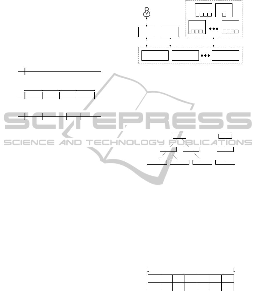
timestamp
start end
step step step step
start t
1
t
2
t
3
(a)
(b)
(c)
Figure 2: Different kinds of schedules: (a) Single schedule
(b) Recurring schedule (c) Module driven schedule.
The analysis cloud should support different kinds
of schedules. In the case of the retailer, the batch
should run from a specific start time to a specific end
time. This recurring schedule should also contain a
step size, which denotes how much time there is be-
tween consecutive timestamps. The analysis cloud
should also have the notion of a single schedule,
which executes a module only for a single timestamp.
Finally, it should be possible to have a schedule that
depends on the sensor data at hand, e.g. to schedule
based on the sample frequency. This leads to the need
for a module driven schedule in which it is left to the
module to decide what the next timestamp should be.
See Figure 2 for a comparison of the different kinds
of schedules.
4 ARCHITECTURE OF THE
ANALYSIS CLOUD
The requirements listed in the previous chapter can be
fulfilled with the architecture shown in Figure 3. Each
solid block is a node in the system, either a physical
machine or a virtual machine. The dotted lines denote
a cluster of nodes containing the same kind of func-
tionality. Sections 4.1 to 4.5 describe each component
in more detail and section 4.6 shows how the whole
system fulfills the mentioned requirements.
4.1 Tasks
There are multiple ways to link timers, schedules and
Orchestration
Server 1
Orchestration
Server 2
Orchestration
Server m
Global
Manager
Web
Server
ZooKeeper ZooKeeper ZooKeeper
HTTP
User
Node
Manager 3
W W W
Node
Manager n
W W W W
Node
Manager 1
W W W W
Node
Manager 2
W
Figure 3: Architecture of the Analysis Cloud.
modules. At least one timer is always available (the
live timer) and there are possibly several simulation
timers. The number of schedules is typically in the
order of dozens, i.e. a bit higher than the number of
timers. Finally, the number of modules is anywhere
from a handful to a few thousand. Figure 4 shows
an example of two timers, three schedules and four
modules and their relationships.
Timer 1
Schedule 1.1 Schedule 1.2
Module 1.1.1 Module 1.1.2 Module 1.2.1
Timer 2
Schedule 2.1
Module 2.1.1
Figure 4: Hierarchy of Timers, Schedules and Modules.
The nodes executing the modules need to know in
which order and from which timestamp each module
should be executed. To keep track of this, there is
the notion of tasks and a work queue containing these
tasks. When a module enters the system, its first exe-
cution time is noted and the combination of this time-
stamp and a reference to the module is placed in the
work queue. The tasks in the work queue are sorted
by timestamp which means that the system can sleep
until the timestamp at the front of the work queue has
passed. The corresponding module is then executed
and the new timestamp (if any) is determined, based
on the module’s linked schedule and timer.
t
1
mod A
t
2
mod B
t
4
mod A
t
5
mod C
t
7
mod A
t
7
mod D
...
...
Front Back
Figure 5: Work queue containing Tasks.
See Figure 5 for an example of a work queue con-
taining tasks. Each black task is currently present, ev-
ery grey one will be added as soon as its black coun-
terpart has finished. In this example, the task for mod-
ule A at timestamp t
4
is added as soon as the execu-
tion of the module at timestamp t
1
has finished. The
same applies to t
7
in combination with t
4
for the same
module.
AnalysisCloud-RunningSensorDataAnalysisProgramsonaCloudComputingInfrastructure
361
4.2 Managers and Workers
A node manager is a necessary part of every comput-
ing node. Each node manager supervises a part of the
work of the total analysis cloud. The actual execu-
tion of the modules is performed by workers. Each
worker listens to the work queue of the node manager
and fetches a task as soon as one becomes available.
Using multiple workers can speed up the processing
when there is more than one processor core available
or one analysis module is fetching data while another
is using the processor. Typically there are two or more
node managers present in the system, and one or more
workers per node manager.
A node manager has two main functions. Its first
function is supervising the execution of user mod-
ules. It uses its work queue containing tasks to de-
cide which modules should be executed at what time.
Its second function is to listen for additions, deletions
and changes in the desired configuration of timers,
schedules and modules. Based on this information,
it makes changes in its internal configuration and re-
ports on its current configuration.
There is a single global manager present in the
system, which coordinates the work among all node
managers. It listens to requests for changes in the total
configuration of the system, i.e. the timers, schedules
and modules. Based on this information it distributes
the work among the node managers. It also listens to
the current configuration of each node manager and
reports on the combined configuration.
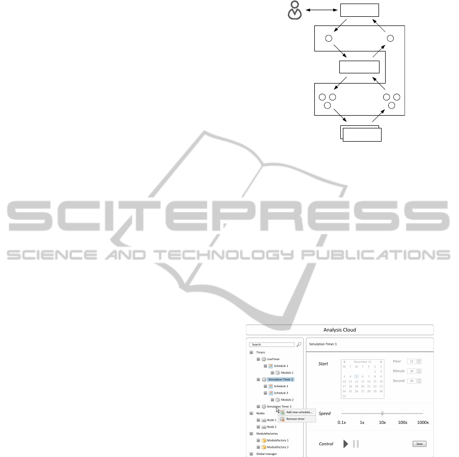
4.3 Orchestration
Except for the communication between the user and
the web server, all communications between com-
ponents of the analysis cloud are performed through
an orchestration system. The ZooKeeper distributed
coordination service (Hunt et al., 2010) (ZooKeeper
Website, 2012) is used for the implementation of this
part of the analysis cloud.
Figure 6 shows how the orchestration works for
the communication of configuration data inside the
system. Starting at the top, the user sets a desired
global configuration, which is a combination of in-
formation about timers, schedules and modules. This
information is automatically picked up by the global
manager, which translates the global desired config-
uration into smaller parts, one for each node man-
ager. The node managers automatically pick this up
and use the configuration data to change their internal
state. This state is then set in the current configura-
tion of each node manager. The global manager auto-
matically picks up these configurations and translates
desired
global
desired
nodes
current
nodes
current
global
WebserverUser
Global Manager
Node Manager
Orchestrati
o
n
Node Manager
Figure 6: Orchestration. Each circle is a key/value pair con-
taining configuration information.
them into a global current configuration. The result of
this is presented to the user.
4.4 Web Interfaces
There are two web interfaces present in the platform.
One is a RESTful (Fielding, 2000) interface that uses
the orchestration system to set the desired configura-
tion of the analysis cloud and read its current con-
figuration. It contains methods for listing all timers,
schedules and modules, and methods to create and re-
move individual instances of those.
Figure 7: Website intended for the users of the Analysis
Cloud and the developers of analysis modules.
The other interface is a set of web pages intended
for users of the analysis cloud and the developers of
analysis modules. Figure 7 shows the design of the
website. The current hierarchy of timers, schedules
and modules is shown on the left side of the screen,
while the right side shows information on the cur-
rently selected item. At the moment, the right mouse
key is pressed and a pop-up menu is shown to add a
schedule to the simulation timer or remove the timer
altogether.
CLOSER2013-3rdInternationalConferenceonCloudComputingandServicesScience
362

4.5 Programming Interfaces
The analysis cloud and its modules are written in Java.
The developer of a module must implement a factory
that is able to create a module with supplied parame-
ters. The mandatory interface for factories looks like
this:
Module create(
Map<String, String> parameters);
When the create function is called, the factory must
create a new module and configure it with the sup-
plied parameters, e.g. by using setters on the module.
Modules must also adhere to a specific interface
to be used on the analysis cloud:
void init(long timestamp);
void execute(long timestamp);
long next();
void terminate();
The init function is called just after the module has
been constructed by the factory. The timestamp pa-
rameter tells the module which timestamp will be
used for the first execution. This helps the module
in its initialization, e.g. by being able to pre load
data from an external source. The execute function
is called one or more times after that for ascending
timestamps. If the module driven schedule is used, the
next function is called after each execution, to ask the
module at which timestamp it would like to be sched-
uled again. Finally, the terminate function is called
when the module is no longer needed, e.g. when the
schedule has finished or the user deletes the module
from the system.
Table 1: Callback functions with the number of calls to each
function for the different types of schedule.
Single
Sched-
ule
Recur-
ring
Sched-
ule
Module
Driven
Sched-
ule
init 1 1 1
execute 1 s
a
m
b
next 0 0 m
b
terminate 1 1 0 or 1
c
a
depends on schedule: ⌊
end−start
step
+ 1
b
depends on module: [0, ∞]
c
depends on module
Table 1 lists the four callback functions of a mod-
ule and shows how many times each function will be
called for each type of schedule.
4.6 Fulfillment of Requirements
Section 3.1 states that there should not be a critical
single point of failure in the system. Iterating through
the components of the analysis cloud shows that this
requirement is fulfilled by the following system fea-
tures:
• If an orchestration server fails, the clients auto-
matically connect to one of the remaining servers.
Since all orchestration servers contain the same
configuration data, there is no loss in functional-
ity.
• If one of the node managers fails, the global man-
ager will redistribute the work among the remain-
ing node managers. A part of the work that the
failed node manager has performed may be per-
formed again by the node manager that took over.
• If the web server fails, the user is unable to mon-
itor and control the analysis cloud. However, the
node managers will continue with the currently
configured work.
• If the global manager fails, the node managersstill
continue with the work they were given. Any up-
dates the user provided on the website are post-
poned until the global manager is restarted.
Section 3.2 states that it should be easy for developers
to create modules for the analysis cloud. Only two in-
terfaces are mandatory, one for the factory and one for
the module. The factory interface contains only one
function and the module interface contains four func-
tions, a compromise between ease of implementation
and performance.
Finally, section 3.3 shows that it is necessary to
have a notion of time that may differ from the ac-
tual, current time. For this purpose, the analysis cloud
provides zero or more user-defined simulation timers
with their own independent time and speed. The plat-
form also provides three types of schedules to support
multiple use cases.
5 EXPERIMENTS ON THE
ANALYSIS CLOUD
Two experiments are performed to show how the anal-
ysis cloud behaves in practice. The first experiment,
described in Section 5.1, shows that the platform is
capable of running multiple modules with the same
schedule. Modules started at a later time gradually
catch up with the modules that were started earlier,
without overloading the system. The second exper-
iment, described in Section 5.2, shows that the plat-
AnalysisCloud-RunningSensorDataAnalysisProgramsonaCloudComputingInfrastructure
363
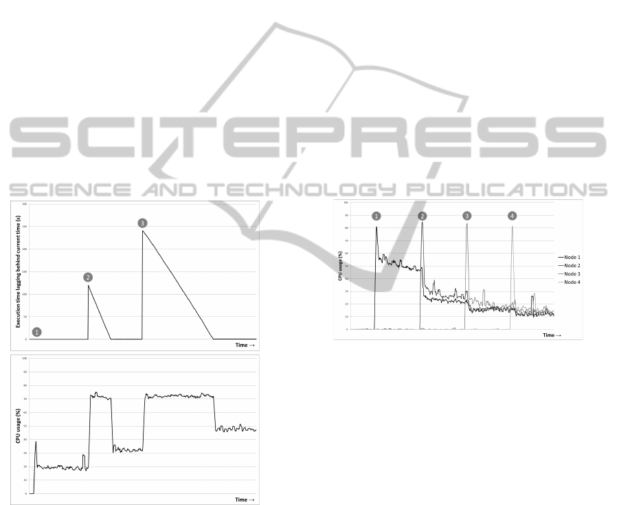
form is capable of distributing its workload over mul-
tiple computing nodes. Adding nodes to the system
results in a shift of some tasks from the old nodes to
the new ones.
5.1 Single Node
An external data source serves sensor data through a
web interface. A single module fetches data from this
web interface in its execute function and performs var-
ious calculations on the data, taking roughly 150 to
200 milliseconds. A recurring schedule is used with
a step size of one second and a simulation timer with
normal speed.
At the start of the experiment, a single module
is created. Two minutes later, a second module is
started with the same schedule and four minutes from
the start a third module is started, also with the same
schedule. Each module uses its own set of input and
output sensor values. A single node manager is ac-
tive during this experiment to be sure that all module
executions take place on the same machine.
Figure 8: Result of the single node experiment. The top
chart shows the number of seconds the timestamp for the
module execution lags behind the actual time. The bottom
chart shows the corresponding CPU usage.
Figure 8 shows the results of the experiment. The
first module is started at moment 1. A small peak
in the CPU load is seen, followed by a steady line at
about 20 percent.
The second module is started at moment 2. The
schedule and its timer were started when the first
module was created, which means that the current
time is now two minutes (120 seconds) ahead of the
start time of the schedule and the module is executed
repeatedly to catch up. This leads to a CPU usage of
about 75 percent until the time gap is gone and the
CPU usage drops to about 35 percent.
The third module is started at moment 3. The gap
between the current time and the timestamp used for
the execution of the module is now four minutes (240
seconds). Catching up now takes even more time, not
only because of this larger gap, but also because the
system now runs three modules instead of two. This
again leads to a CPU usage of about 75 percent until
the time gap is gone and the CPU usage drops to about
50 percent.
5.2 Multiple Nodes
Multiple computing nodes are active in the analysis
cloud during this experiment. At the start of the ex-
periment, a large number of modules is configured
and a single node is started. Two minutes later a sec-
ond node is started, four minutes later a third, and six
minutes later a fourth.
Figure 9: Result of the multiple nodes experiment. The
chart shows the CPU usage over time as nodes are added to
the analysis cloud.
Figure 9 shows the results of the experiment. The
first node is started at moment 1. A peak in the CPU
usage is seen, followed by a fairly steady line of about
50 percent. The CPU usage of the other (inactive)
nodes is then still about 0 percent.
The second node is started at moment 2. At that
moment the global manager redistributes the modules
among both node managers, which results in a lower
CPU usage of node 1. The CPU usage of node 2 is
roughly the same, about 25 percent. The same applies
to moments 3 and 4 where a third and a fourth node
are started. The CPU usage of all four nodes is then
roughly the same at about 15 percent.
6 CONCLUSIONS
Several platforms and frameworks exist for the anal-
ysis of data. However, none of the currently existing
CLOSER2013-3rdInternationalConferenceonCloudComputingandServicesScience
364

solutions is tailored for the needs of sensor data anal-
ysis.
This paper presents a system that supports the pro-
cessing of both live sensor data feeds and batches of
historical sensor data. It contains simulation timers
and different schedules including single, recurring
and module driven. Moreover, the analysis cloud has
simple programming interfaces, which makes it easy
to develop analysis modules.
Experiments demonstrate that the system is capa-
ble of running analysis modules in a robust manner,
and can catch up quickly when there is a discrepancy
between the timestamp for an execution of a module
and the actual time. Also, the capacity of the analysis
cloud can be scaled up or down on demand by adding
or removing computing nodes from the system.
The current analysis cloud leaves the actual re-
trieval and storage of sensor data to the module, i.e.
each module must communicate with an external stor-
age system before and after it performs calculations
on the sensor data. It is therefore possible that mul-
tiple modules extract the same data from the storage
system. In a future version of the analysis cloud, we
would like to avoid the cost of this redundantretrieval.
The experiments in this paper are limited in scale
and time. Using the analysis cloud for a longer period
of time, with a larger number of nodes, will result in
better understanding of its features and weaknesses.
In future work we would like to assess this usage to
better answer questions about scalability and limiting
factors.
ACKNOWLEDGEMENTS
This publication is supported by the Dutch national
programs Flood Control 2015 and COMMIT.
REFERENCES
Akka Website (2012). Akka toolkit for event-driven appli-
cations on the jvm. http://akka.io.
Blackwell, W. (2005). A neural-network technique for
the retrieval of atmospheric temperature and moisture
profiles from high spectral resolution sounding data.
IEEE Transactions on Geoscience and Remote Sens-
ing.
Dean, J. and Ghemawat, S. (2004). Mapreduce: Simpli-
fied data processing on large clusters. Symposium on
Operating Systems Design and Implementation.
Disco Website (2012). Disco distributed computing frame-
work. http://discoproject.org.
Esper Website (2012). Esper complex event processing.
http://esper.codehaus.org.
Fielding, R. T. (2000). Architectural styles and the design
of network-based software architectures. http://
www.ics.uci.edu/∼fielding/pubs/dissertation/fielding
dissertation.pdf.
Ghemawat, S., Gobioff, H., and Leung, S.-T. (2003). The
google file system. ACM Symposium on Operating
Systems Principles.
Hadoop Website (2012). Apache hadoop. http://
hadoop.apache.org.
Hunt, P., Konar, M., Junqueira, F. P., and Reed, B. (2010).
Zookeeper: Wait-free coordination for internet-scale
systems. USENIX Annual Technical Conference.
IBM Corporation (2001). Autonomic computing: Ibms
perspective on the state of information technology.
http://www.research.ibm.com/autonomic/manifesto/
autonomic computing.pdf.
Munish, K. G. (2012). Akka Essentials. Packt Publishing.
Neumeyer, L., Robbins, B., Nair, A., and Kesari, A. (2010).
S4: Distributed stream computing platform. IEEE In-
ternational Conference on Data Mining Workshops.
Pyayt, A., Mokhov, I., Lang, B., Krzhizhanovskaya, V., and
Meijer, R. (2011). Machine learning methods for en-
vironmental monitoring and flood protection. Interna-
tional Conference on Artificial Intelligence and Neu-
ral Networks.
Rao, J., Bu, X., Xu, C.-Z., and Wang, K. (2011). A dis-
tributed self-learning approach for elastic provision-
ing of virtualized cloud resources. IEEE International
Symposium on Modelling, Analysis, and Simulation of
Computer and Telecommunication Systems.
S4 Website (2012). S4 distributed stream computing plat-
form. http://incubator.apache.org/s4.
Sheng, B., Li, Q., and Mao, W. (2006). Data storage place-
ment in sensor networks. ACM International Sympo-
sium On Mobile Ad Hoc Networking and Computing.
Spark Website (2012). Spark cluster computing framework.
http://www.spark-project.org.
Storm Website (2012). Storm distributed realtime compu-
tation system. http://storm-project.net.
White, T. (2009). Hadoop: The Definitive Guide. O’Reilly
Media.
Zaharia, M., Chowdhury, M., Franklin, M. J., Shenker, S.,
and Stoica, I. (2010). Spark: Cluster computing with
working sets. HotCloud.
ZooKeeper Website (2012). Apache zookeeper. http://
zookeeper.apache.org.
AnalysisCloud-RunningSensorDataAnalysisProgramsonaCloudComputingInfrastructure
365
